Excel Efficiency: Most Used Excel Functions

Embarking on mastering Excel functions can transform your data analysis and productivity. Ever wondered which Excel functions are absolute game-changers?

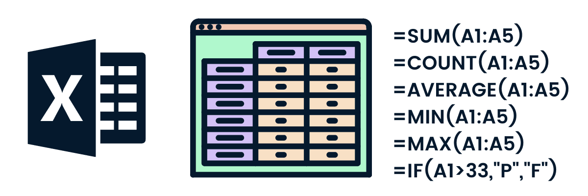
 Let's explore Excel, where functions like SUM, SUBTOTAL, and CONCAT can revolutionize data handling. Imagine seamlessly summarizing rows of numbers with SUM, delving deep into your data with SUBTOTAL's versatile calculations, or merging information creatively with CONCAT. 

But wait, there's more! Are you ready to take an interactive journey into the world of Excel? Let's explore these indispensable tools together and unlock new levels of efficiency and insight in your Excel adventures​​.

Most Used Excel Functions

Here is our list of the most used Excel functions:

1. SUM Function
2. SUBTOTAL Function
3. CONCAT Function
4. IF and IFS Functions
5. VLOOKUP and HLOOKUP Functions
6. COUNTIF and COUNTIFS Functions
7. AVERAGE, MEDIAN, and MODE Functions
8. TEXT Functions (LEFT, RIGHT, MID)
9. XLOOKUP Function
10. PivotTables and Excel Functions
11. Dynamic Arrays (FILTER, SORT, UNIQUE)
12. Error Handling (IFERROR, ISERROR)

Let's dive in!

SUM Function

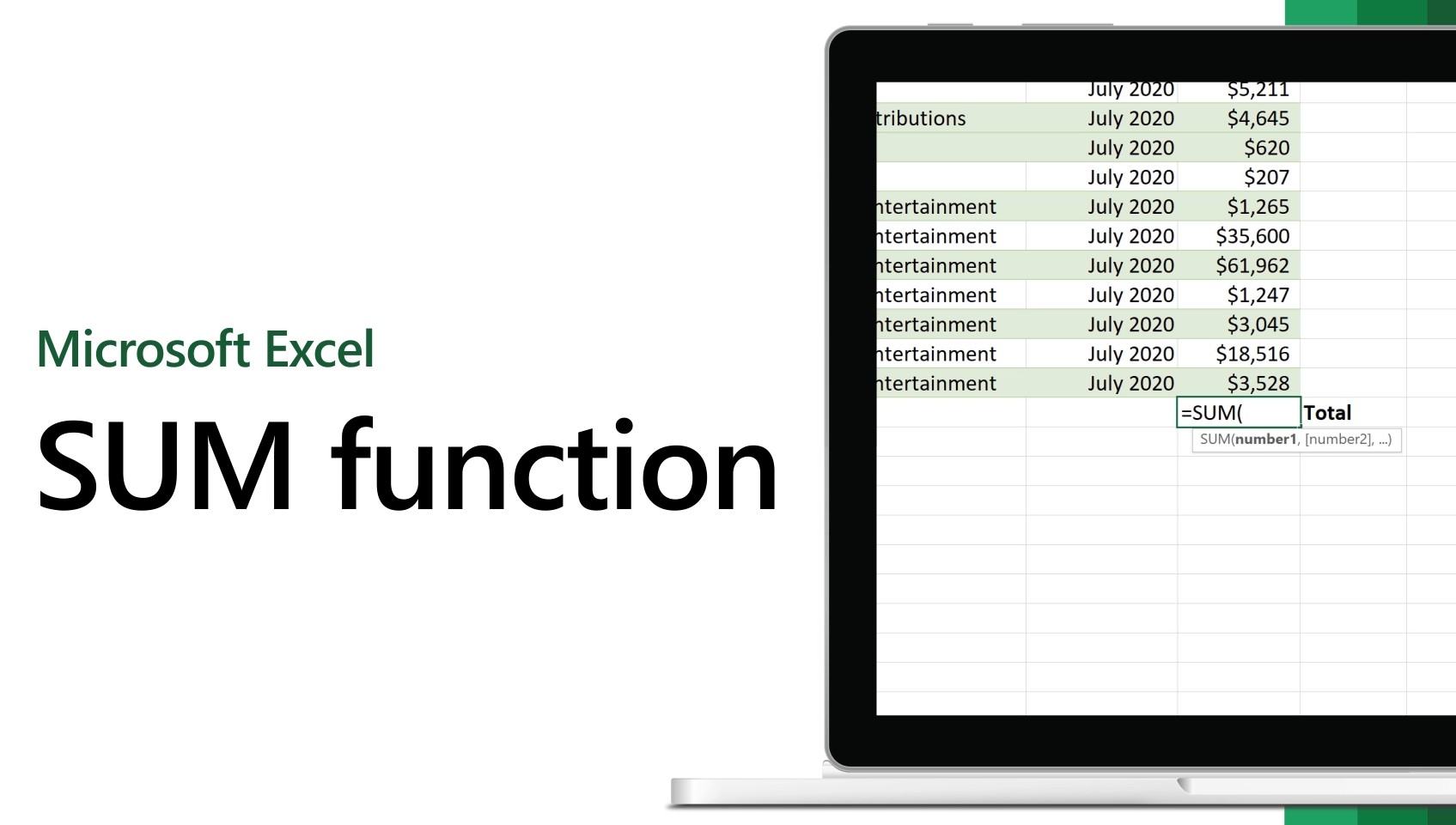
The SUM function in Excel is a fundamental tool that significantly enhances data analysis and productivity in various sectors, particularly in business and finance. This function allows users to quickly aggregate a series of numbers, cell references, ranges, arrays, constants, or the results of other formulas, providing a total sum. 

It supports up to 255 arguments, making it versatile for diverse calculations.

In business and finance, the SUM function can be pivotal for calculating total sales, expenses, revenue, or any financial metric over a given period. For example, a business may use the SUM function to determine the total sales for the year's first six months or to sum up expenses in different categories to get an overall view of financial outflow.

Furthermore, using the ROUND function, the SUM function can be nested within other functions to perform more complex calculations, like rounding off the total sum to a specific number of decimal places. This ability to nest functions expands the utility of the SUM function, enabling intricate calculations within a single cell​​.

However, it's essential to be aware of some limitations and considerations when using the SUM function. For instance, the function will return an error if the range includes error values. 

In such cases, combining SUM with the IFERROR function can help by substituting zero for any errors within the range, thus allowing the summation to proceed without interruption​​.

SUBTOTAL Function

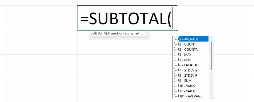
The SUBTOTAL function in Excel is a versatile tool that goes beyond simple addition, offering various calculations like sum, average, count, and more, depending on the function number you choose. It's particularly useful in scenarios like inventory management because it allows you to perform these calculations on filtered data, excluding hidden rows, which is a significant advantage when analyzing subsets of data.

For instance, if you have a list of inventory items with their quantities and prices, you can apply filters based on categories or time frames and use the SUBTOTAL function to calculate totals or averages only for the visible, filtered data. This capability is invaluable for getting quick insights into specific inventory segments without creating separate tables or lists.

The SUBTOTAL function has 1-11 and 101-111 numbers. The former includes hidden cells in its calculations, whereas the latter excludes them, providing flexibility based on your needs. 

This dual functionality allows you to adapt the function to various scenarios, such as adjusting your inventory analysis based on visible data points or considering the entire dataset, including hidden rows​​.

In practice, you could use SUBTOTAL to calculate the total stock value of filtered items, the average price of visible products in a category, or count the number of items in stock within a specific range, adjusting dynamically as filters are applied or removed. This function is not just limited to summing; it can apply any of its 11 different calculations to your filtered inventory data, offering a comprehensive tool for data analysis within Excel​​.

CONCAT Function

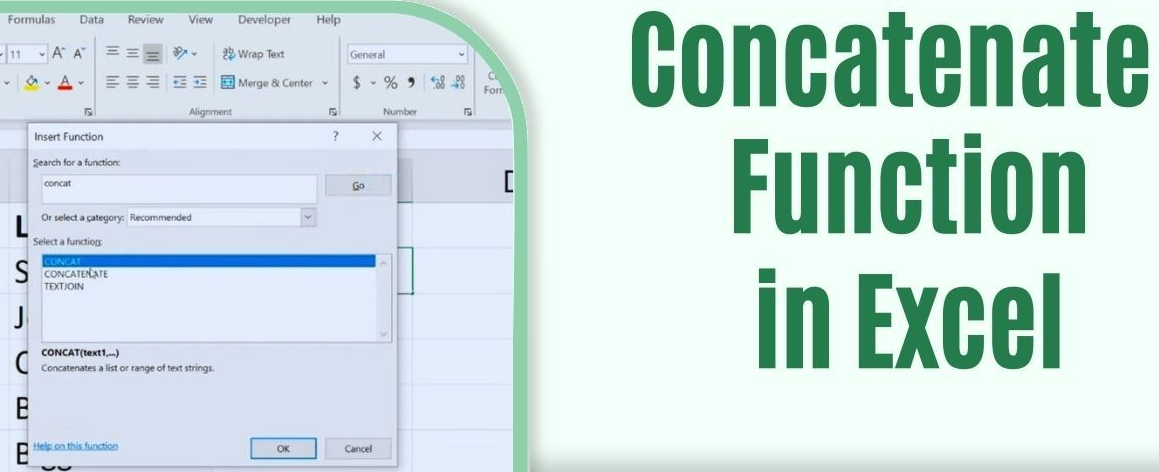
The CONCAT function in Excel is designed for merging text from multiple cells or ranges, creating comprehensive data strings. It's a powerful tool introduced in Excel 2016 as an enhancement over the older CONCATENATE function. 

The CONCAT function can handle a range of cells, not just individual cell references, which makes it more efficient for combining large data sets.

For example:

If you want to merge the first and last names from different cells with a space between them, you will use =CONCAT(A1, " ", B1). This function can also handle different delimiters, such as commas or line breaks, between the text elements you combine. 

If you needed to add a comma and space between words, your formula might look like =CONCAT(A2, ", ", B2, ", ", C2).

One of CONCAT's key benefits is its ability to ignore empty cells automatically. This feature simplifies merging text from ranges that might have gaps. 

However, it's essential to remember that CONCAT doesn't provide a built-in way to specify a delimiter for the combined values, unlike the TEXTJOIN function, which can be used when a common delimiter is needed.

In addition to text, CONCAT can be used to merge numerical values and dates, though it's crucial to use the TEXT function to maintain proper formatting for numbers and dates within the CONCAT formula. For instance, to merge text and a formatted date, you might use =CONCAT("The date is ", TEXT(A1,"mmmm d")).

In inventory management:

CONCAT can be incredibly useful for creating unique identifiers or detailed descriptions by combining information from multiple columns into one. For example, you could combine product codes, names, and specifications stored in separate columns into a single, detailed product description column.

IF and IFS Functions

The IF and IFS functions in Excel allow you to perform conditional operations. While the IF function tests a single condition, the IFS function can evaluate multiple conditions sequentially.

Here's a comparative table that outlines the key differences and uses of the IF and IFS functions in Excel:

The IF function is ideal when you have a single condition to test or when you want specific control over each logical test's outcomes. In contrast, the IFS function is more efficient and easier to read when you have multiple conditions to check, avoiding the complexity of nested IF statements.

VLOOKUP and HLOOKUP Functions

Excel's VLOOKUP and HLOOKUP functions in Excel are designed for vertical and horizontal data retrieval. Here's a detailed breakdown of their functionalities and importance in data retrieval:

VLOOKUP is widely used in various vertical lookup applications, especially when dealing with tabular data where specific information needs to be extracted based on a matching condition. HLOOKUP serves a similar purpose but is designed for horizontal data layouts, making it a crucial tool for retrieving information across rows. 

Both functions are fundamental for data analysis, reconciliation tasks, and streamlining data manipulation processes in Excel.

COUNTIF and COUNTIFS Functions

Excel's COUNTIF and COUNTIFS functions in Excel are essential for conducting conditional counting in datasets, such as customer data analysis.

Here's an overview of how they work and how they can be applied in a practical context:

• COUNTIF Function in Excel: COUNTIF counts the number of cells that meet a specific criterion within a range. Its syntax is =COUNTIF(range, criteria). The function is versatile, allowing you to use logical operators (e.g., >, <, =) for numeric data and wildcard characters (e.g., *, ?) for text data​​.
• COUNTIFS Function in Excel: COUNTIFS extends the capabilities of COUNTIF by allowing you to apply multiple criteria across multiple ranges. Its syntax is =COUNTIFS(criteria_range1, criteria1, [criteria_range2, criteria2], ...). This function is particularly useful when you must simultaneously analyze data based on several conditions​​.

Application in Customer Data Analysis:

• Identifying Customer Segments: You can use COUNTIF and COUNTIFS to segment customers based on various attributes. For instance, in a retail banking dataset, you could categorize customers by balance ranges using IF statements and then apply COUNTIF to count the number of customers within each balance band​​.
• Cross-Reference Analysis: With COUNTIFS, you can perform cross-reference analysis by applying multiple criteria. For example, you could analyze the distribution of customer balances across different regions, identifying how many customers have balances above a certain threshold within each region​​.
• Trend Analysis Over Time: By incorporating time-related criteria, COUNTIF and COUNTIFS can help you analyze trends over time, such as tracking the growth or decline of customer accounts or analyzing regional performance across different periods​​.
• Handling Text and Dates: These functions are adept at handling text and dates. For example, COUNTIF can be used to count occurrences of a specific name within a data range, and with dates, you can use COUNTIFS to count occurrences before or after a certain date or within a date range​​.

AVERAGE, MEDIAN, and MODE Functions

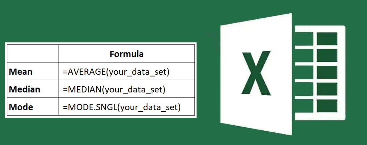
The functions AVERAGE, MEDIAN, and MODE in Excel are fundamental for statistical analysis, particularly in market research or sales data analysis. Here's a summarized table outlining their use cases:

For example, the AVERAGE function can help analyze average customer satisfaction scores in market research. The MEDIAN function is beneficial when you want to find the middle point in data, like the median sale price, which can provide insights without being skewed by extremely high or low values. 

The MODE function can be crucial in identifying consumers' most common preferences or choices, such as their most preferred product features.

TEXT Functions (LEFT, RIGHT, MID)

Excel's LEFT, RIGHT, and MID functions are powerful tools for manipulating text strings, which can be extremely useful in data cleaning and organization tasks. Here's a brief overview of how these functions can be applied:

• LEFT Function: The LEFT function extracts a specified number of characters from a text string's beginning (left side). For example, if you have a string 'ABCDEF' and use =LEFT("ABCDEF",3), the result will be 'ABC'​​.
• RIGHT Function: Conversely, the RIGHT function extracts characters from a text string's end (right side). Using the same string 'ABCDEF' with =RIGHT("ABCDEF",3), the result will be 'DEF'​​.
• MID Function: The MID function extracts characters from the middle of a text string, given a starting position and the number of characters to extract. For instance, =MID("ABCDEF",2,3) would result in 'BCD', starting from the second character and extracting three characters in total​​.

These functions can be particularly useful in various scenarios, such as:

• Extracting specific parts of data entries that follow a consistent pattern (e.g., extracting area codes or extensions from phone numbers).
• Isolating specific information from strings where identifiable characters or patterns surround the desired text.
• Cleaning data by removing unnecessary prefixes or suffixes in strings.

For example, in data cleaning, you might encounter a situation where you must extract just the first name from a full name. If the full name is in the format 'First Last', you could use the LEFT function and FIND to extract the first name. 

Similarly, the MID function can be invaluable if you need to extract data consistently positioned in the middle of strings.

XLOOKUP Function

XLOOKUP is a powerful Excel function introduced as a more flexible and potent alternative to the older VLOOKUP and HLOOKUP functions. The XLOOKUP function searches a range or an array, and then returns the item corresponding to the first match it finds. If no match exists, then XLOOKUP can return the closest (approximate) match. *If omitted, XLOOKUP returns blank cells it finds in lookup_array.

Here's an overview of how XLOOKUP can enhance your data analysis tasks:

1. Simpler Syntax: XLOOKUP requires only three essential arguments: the lookup value, the lookup array, and the return array. This streamlined approach makes it easier to use compared to its predecessors​​.
2. Bidirectional Lookups: Unlike VLOOKUP, which only searches in a left-to-right direction, XLOOKUP can retrieve data to the left or right of the lookup values, offering greater flexibility​​.
3. Enhanced Match Control: XLOOKUP allows for exact matches, approximate matches, and even wildcard matches, providing more control over how your searches are conducted​​.
4. Custom Error Handling: If XLOOKUP doesn't find a match, you can specify a custom return value, which simplifies error handling in your formulas​​.
5. Versatility in Return Values: XLOOKUP can return single values, arrays, or entire rows/columns, expanding its utility in various scenarios​​.
6. Search Modes: You can define the direction of the search, either from the first to the last value or in reverse, adding another layer of flexibility to your lookup tasks​​.

Here are a couple of practical examples where XLOOKUP can be particularly useful:

• Dynamic Two-Way Lookups: XLOOKUP can perform vertical and horizontal lookups in a single formula, making it an excellent tool for two-way lookups where you need to find a value at the intersection of a specific row and column​​.
• Nested XLOOKUP for Multiple Data Sets: You can nest XLOOKUP functions to search across multiple data sets, even on different sheets, which is particularly useful when consolidating data from various sources​​.

PivotTables and Excel Functions

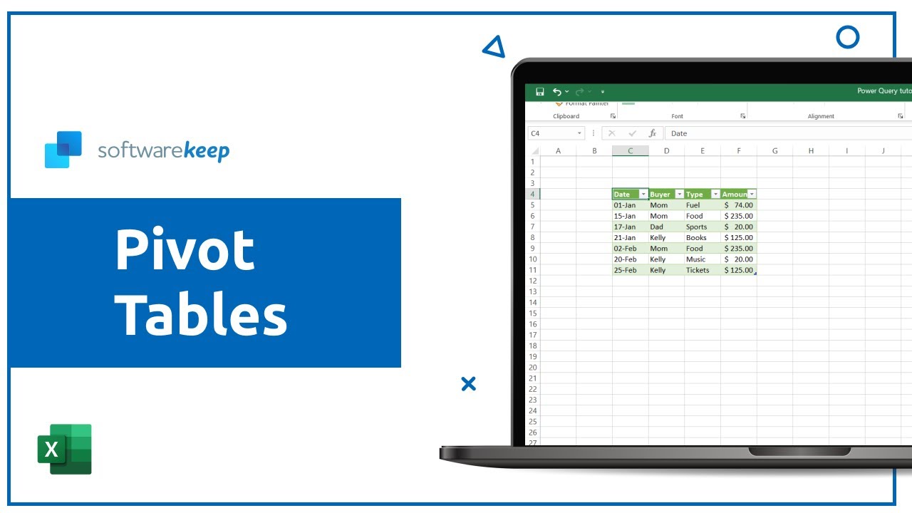
Various Excel functions can significantly enhance PivotTables in Excel, making complex data analysis simpler and more intuitive. Here are some ways to enhance PivotTables with Excel functions and examples of how they can simplify complex data analyses:

1. Slicers for Data Segmentation: Slicers provide a quick way to filter PivotTable data interactively. By adding a slicer, you can filter the data displayed in the Pivot Table based on your selection, making it easier to focus on specific data segments​​.
2. Calculated Fields: You can create calculated fields within PivotTables to perform calculations on your data. For instance, if you're analyzing sales data, you can create a calculated field to determine the profit for each item by subtracting the cost from the sales price​​.
3. Multiple Pivot Tables from One Source: You can create multiple pivot tables from a single data source to analyze different aspects of your data. This can be particularly useful for comparing different data segments side by side​​.
4. Advanced Sorting and Filtering: PivotTables allow for advanced sorting and filtering, including custom sorting and the ability to filter by top 10 values or specific ranges. This makes it easier to focus on your analysis's most relevant data points ​​.
5. Timeline Filtering: If your data includes date fields, you can add a timeline to your PivotTable, allowing you to easily filter data based on periods. This is especially useful for time-based data analysis, such as sales trends​​.
6. Value and Label Filtering: Beyond the basic filtering options, PivotTables support more nuanced filtering techniques, such as value and label filters, enabling you to narrow down your data precisely based on specific criteria or conditions​​.

Dynamic Arrays (FILTER, SORT, UNIQUE)

Excel's dynamic array functions, FILTER, SORT, and UNIQUE, offer powerful data segmentation and organization tools. Here's a brief overview of how these functions can be applied in practical scenarios:

These functions allow for advanced data manipulation in Excel, providing efficient ways to dynamically segment, sort, and extract unique values from your data.

Error Handling (IFERROR, ISERROR)

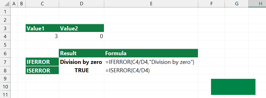
In Excel, the IFERROR and ISERROR functions are pivotal for managing calculation errors, thereby maintaining data integrity. In its pure form, ISERROR just tests if the value is an error or not. It's available in all Excel versions. The IFERROR function is designed to suppress or disguise errors - when an error is found, it returns another value that you specify.

Here's an overview of how these functions work and their applications:

• IFERROR Function: This function allows you to specify a custom output when a formula detects an error. Its syntax is =IFERROR(value, value_if_error), where value is the evaluated expression, and value_if_error is the result returned if an error is detected.
  For example, =IFERROR(1/0, "Error") would return "Error" instead of the default #DIV/0! error. This function is particularly useful for ensuring that your spreadsheets remain clean and user-friendly, avoiding the clutter of standard error messages.
  It's also commonly used with VLOOKUP to handle the #N/A error when a lookup value isn't found​​.
• ISERROR Function: This function determines if a formula results in an error, returning TRUE if there's an error and FALSE otherwise. Its usage is straightforward: =ISERROR(value) checks if value is an error.
  This function is especially useful for preemptively checking for errors across a range of cells. For instance, =ISERROR(1/0) would return TRUE. You can combine ISERROR with IF to provide a specific output when an error is detected, like =IF(ISERROR(1/0), "Error detected", 1/0), which would return "Error detected" in case of an error​​.

These functions are essential for maintaining data integrity and readability in practical applications, especially in large datasets where manual error checking is impractical. They are used in various scenarios, such as financial analysis, inventory management, and data validation processes, to ensure accurate and error-free results.

Final Thoughts

Mastering the IFERROR and ISERROR functions in Excel is crucial for anyone aiming to enhance their spreadsheet skills. These functions are key to managing errors efficiently, ensuring data integrity, and maintaining spreadsheet readability. 

By incorporating IFERROR and ISERROR into your Excel toolkit, you can handle unexpected inputs gracefully and keep your data analysis processes robust and error-free. Now that you understand the importance of these functions, explore them further and boost your Excel proficiency. 

Whether you're a beginner or looking to refine your skills, delving into these functions will elevate your spreadsheet game.

Keep Learning

» How To Use Excel’s DATE Formula Function
» Excel Tutorial for Beginners: Tips You Need to Know
» How to Manage Your Finances With Microsoft Excel
» The Benefits of Microsoft Office for Students and Professionals
» Office 2021 for Home and Business Guide