Are you struggling to visualize your data in Excel charts effectively? If so, learning how to switch rows and columns in Excel can make a big difference.
In this article, we'll show you how to do just that, step by step.
So let's start and take your Excel skills to the next level.
Table of Contents
- What is an Excel chart?
- Change the way that data is plotted
- How to access the "Select Data" option in Excel
- How to modify an Excel chart
- Different types of Excel charts
- Tips for effective Excel charting
- FAQs
- Final Thoughts
What is an Excel chart?
Excel charts are like pictures that show information in a way that's easy to understand. They're made with Microsoft Excel, which organizes and calculates numbers.
When you make a chart in Excel, it turns your numbers into pictures. These pictures can show how much money you earned or how many pets you have.
There are different kinds of charts that you can make in Excel.
For example:
There are bar charts that look like tall rectangles and show how much of something you have.

There are also line charts that show how something changes over time.
For example:
A line chart could show how much a plant grows weekly.

Excel charts are helpful because they let you see your information in a way that's easy to understand. Instead of looking at a big list of numbers, you can look at a picture that shows the same information. That's why charts are often used in schools and businesses to help people make decisions.
Change the way that data is plotted
One thing you can do is change which information is plotted on each axis.
- Click on your chart. This will make some new tabs appear at the top of the screen. These tabs are called Chart Tools, and they let you change how your chart looks.
- Click on the Design tab. This is where you can find the button that lets you switch which information is on which axis. It's called "Switch Row/Column" in the Data group.

When you click "Switch Row/Column," your chart will change to show the information differently.
For example:
If your chart shows how much money you made each month, it might show how much you made each year instead. This can make understanding your information and seeing patterns in your data easier.
How to access the "Select Data" option in Excel
To access the "Select Data" option in Excel, you need to follow these steps:
- Go to the "Insert" tab at the top of your Excel window.
- Select the type of chart that you want to create. You can choose from different chart types such as column, line, or pie chart.
- Once you have selected your chart type, you will see a new tab called "Chart Design" at the top of the window.
- Click on the "Chart Design" tab, and you will see a button called "Select Data" in the "Data" group.
-
Click on the "Select Data" button, and a new window will appear.

-
In the "Chart data range" box, select the data in your worksheet that you want to use for your chart.

- Once you have selected your data, click the "OK" button to create your chart.
By following these steps, you can easily access the "Select Data" option in Excel and create charts that visualize your data clearly and meaningfully.
How to modify an Excel chart
Modifying an Excel chart is a simple process that can help you to present your data more effectively. If you need to edit or rearrange a series in your chart, you can follow these steps:
- Rright-click on your chart to open the chart menu.
- Select "Select Data" from the menu.
- In the "Legend Entries (Series)" box, you will see a list of the data series included in your chart. Click on the series that you want to modify.
- Click on the "Edit" button to open the "Edit Series" window.
- In the "Series name" field, you can modify the name of the series if needed.
-
In the "Series values" field, you can modify the range of cells that are used to create the series.

- Click on "OK" to save your changes.
If you need to rearrange a series, you can select it in the "Legend Entries (Series)" box, and then click on the "Move Up" or "Move Down" buttons to change its position in the chart.
By following these steps, you can easily modify and customize an Excel chart to meet your needs. This can help you to communicate your data more effectively and make more informed decisions based on your data.
Different types of Excel charts
Each chart shows your information in a different way. Here are some types of charts that you can make:
-
Column Chart: This chart is good for showing how much of something you have. For example, you can make a column chart to show how many pets you have.

-
Line Chart: This chart is good for showing how something changes over time. For example, you can make a line chart to show how much a plant grows each week.

-
Bar Chart: This chart is similar to a column chart, but the bars are shown horizontally instead of vertically. It's good for showing comparisons between things.

-
Area Chart: This chart is good for showing how something changes over time, just like a line chart. However, the area under the line is filled in with color. This makes it easier to see the difference between different parts of the chart.

-
Stock Chart: This chart is good for showing how the value of a stock changes over time. It has special features that show the opening price, closing price, and other information about the stock.

By choosing the right type of chart for your information, you can make it easier to understand and see patterns in your data.
Tips for effective Excel charting
Creating an effective chart in Excel can help you visualize your data and make better decisions. Here are some tips to make your charts stand out:
- Choose the right chart type: The first step to creating a good one is to select the correct one. Different types of charts are available in Excel, such as bar charts, line charts, and pie charts. Your chosen chart type will depend on the data you want to represent and the story you want to tell.
- Remove unnecessary axes: When creating a chart, removing any unnecessary axes that don't add value to the chart is important. For example, if you're creating a pie chart, you don't need to include an x or y-axis.
- Distribute bars evenly: If you're creating a bar chart, it's important to distribute them evenly. This makes it easier to compare the data and see any trends.
- Remove background lines: It's best to remove any lines that don't add value to the chart. This can make the chart cleaner and easier to read.
- Keep it simple: Finally, keeping the chart simple and avoiding unnecessary styling is important. This can distract from the data and make the chart harder to understand.
By following these tips, you can create an effective Excel chart that helps you understand your data better.
FAQs
How do you swap columns and rows in Excel?
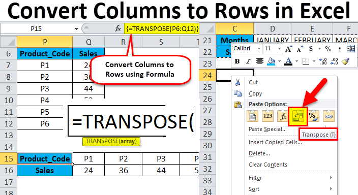
To swap columns and rows in Excel, you can use the "Transpose" feature. Select the data you want to transpose, right-click, choose "Paste Special," and then check the "Transpose" option.
- Select the range of data you want to rearrange, including any row or column labels, and either select Copy.
- Select the first cell where you want to paste the data, and on the Home tab, click the arrow next to Paste, and then click Transpose.
Is there an easy way to flip columns and rows in Excel?
Yes, Excel's "Transpose" feature allows you to easily flip columns and rows by selecting and transposing the data.
How do you switch rows in Excel?
To switch rows in Excel, you can cut the row you want to move, right-click on the target row where you want to switch it, and choose "Insert Cut Cells" to move the row.
How do I switch columns A and B in Excel?
To switch columns A and B in Excel, select both columns, right-click, choose "Cut," right-click on the desired location, and select "Insert Cut Cells" to switch the columns.
How do you shift rows and columns?
To shift rows or columns in Excel, select the rows or columns you want to move, right-click, choose "Cut" or "Copy," right-click on the target location, and select "Insert Cut Cells" or "Insert Copied Cells" to shift them.
Final Thoughts
Switching rows and columns in an Excel chart is a simple process that can help you gain new insights into your data. By following the steps outlined above, you can easily change the orientation of your chart and view your data differently.
This can be particularly useful for comparing multiple data sets or analyzing your data from a new perspective. By experimenting with different chart layouts, you can better understand your data and make more informed decisions.
So don't be afraid to try switching rows and columns in your Excel charts - you may be surprised at what you discover!
One more thing
If you have a second, please share this article on your socials; someone else may benefit too.
Subscribe to our newsletter and be the first to read our future articles, reviews, and blog post right in your email inbox. We also offer deals, promotions, and updates on our products and share them via email. You won’t miss one.