Microsoft Excel is an application with hundreds of tools and endless possibilities. This may be quite intimidating for users just starting out with the software. The tips and tricks below all aim to make your experience using the application better and faster. It doesn’t matter how much experience you have with Microsoft Excel, we’re here to help you increase your productivity and efficiency when creating new projects.
Jump To:
- 1. Add multiple rows and columns at once
- 2. Apply filters to your data
- 3. Remove duplicate entries with one click
- 4. Use conditional formatting
- 5. Import a table from the internet
- 6. Speed up your work process with AutoFill
- 7. Insert a screenshot with ease
- 8. Add checkboxes to your spreadsheet
- 9. Utilize Excel shortcuts
- 10. Remove gridlines from a spreadsheet
- 11. Quickly insert a Pivot Table
- 12. Add comments to your formulas
- 13. Draw your equations
Microsoft Excel Tips and Tricks
Note: The tips below are written for Excel 2016 or later. Earlier versions of Microsoft Excel might require different steps, or have missing features.
Let’s see how you can become a professional Excel user by simply utilizing 13 tips and tricks.
1. Add multiple rows and columns at once
how to insert multiple columns at once in Excel
Spreadsheeting is the most common thing you’ll do in Excel. Whenever creating spreadsheets, you’ll be adding new rows and columns, sometimes hundreds at once. This simple trick makes it easy to do it in a split second, rather than having to add new entries manually.
This is how to add multiple rows or columns at once in Excel.
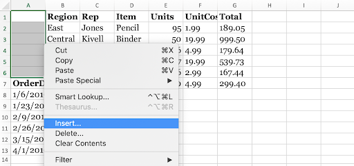
- Highlight the same amount of rows or columns as you want to insert. The rows and columns can have data inside them — this won’t affect the new cells.
- Right-click on any of the selected cells, then click Insert from the context menu.
- The new, empty cells will appear above or to either side of the first cell you originally highlighted. This can be selected.
As you can see in the example below, creating new cells in bulk is extremely easy and will save you time.
2. Apply filters to your data
Filtering which type of item is being shown in an Excel spreadsheet
When working with sets of data, simplifying it may help you see patterns and other crucial information you need. Browsing through hundreds of rows and columns for specific data entries only leaves room for error. This is where Excel’s data filters are a huge help.
As the name suggests, filters help you curate your data and only show you entries fit for specific criteria. For example, if you have a long list of customers but you only want to display people from California, apply a filter. It’ll hide each customer entry that specifies a different location. It’s that easy!
Let’s see how you can implement filters to your Excel spreadsheets.
- Open the spreadsheet you want to filter.
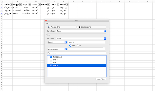
- Click on the Data tab from the Ribbon, and select Filter. This will turn on filtering for your entire spreadsheet, which you can notice by the added drop-down arrows for each header.
- Click on the drop-down arrow for the column you want to filter by. A new window should appear.
- Select how you want your data to be organized. Remove the tick from any heading you don’t want to display and customize how Excel sorts your remaining data.
3. Remove duplicate entries with one click
Remove duplicate cells in Excel
Especially in large sets of data, you might have some unwanted duplicate entries. While it’s possible to manually find these entries, there’s a much faster way to remove them without leaving anything behind. Let’s see how.
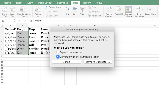
- Highlight the row or column you want to remove duplicates from.
- Open the Data tab from the Ribbon, then click on the Remove Duplicates button under Tools. A new window will appear where you can confirm the data you want to work with.
- Click on the Remove Duplicates button. Voila!
4. Use conditional formatting
Conditional formatting in Excel
Conditional formatting is a huge visual help when you analyze data sets. It changes a cell’s color based on the data within it and the criteria you set. This can be used to create heat maps, color code common information, and much more. Let’s see how you can start implementing this feature into your spreadsheets.
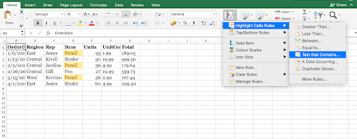
- Highlight the group of cells you want to work with.
- Make sure to be on the Home tab from the Ribbon, then click on Conditional Formatting.
- Select the logic you want to use from the drop-down menu, or create your own rule to customize how Excel treats each cell.
- A new window should open up where you can provide Excel the necessary rules to sort your data properly. When done, click on the OK button and see your results.
5. Import a table from the internet

Insert table from the web in Excel (Source: Analytics Tuts)
Excel allows you to quickly import tables from the internet, without having to worry about formatting or janky cells. Let’s take a look at how you can do this straight from the software itself.
- Switch to the Data tab from the Ribbon, then click on the From Web button.
- In the web browser, enter the website URL that contains the table you want to insert. For example, we’ll be working with an Excel Sample Data table from Contextures.
- Hit the Go button. Once the site loads, scroll down to the table you want to insert.
- Click on the Click to select this table checkbox.
- Click on the Import button.
- Click on OK. The table should appear in your spreadsheet as cells.
6. Speed up your work process with AutoFill
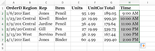
Using AutoFill in Excel
Entering a series of repetitive data gets tedious quite quickly. To combat this, use AutoFill. It’s an extremely simple and easy to implement a feature that recognizes repetitive patterns such as dates, and automatically fills in missing cells. Here’s how to use it.
- Select the cells you want to use as a pattern.
- Hover in the bottom-right corner of a cell until the cursor turns into a black + sign. This indicates the AutoFill feature.
- Click and hold your mouse, then drag the cursor down while holding your click. You should see the predicted data appear as you move the mouse.
- Let go of the mouse when you’re satisfied with the entries.
7. Insert a screenshot with ease
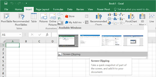
Insert a screenshot into Excel (Source: WebNots)
If you want to include a screenshot of an application you have open, but don’t want to go through the often complicated process of saving one, Excel has your back. Using this simple feature, you can screenshot any active window and immediately insert the taken image into Excel.
To use it, just click on the Insert tab and select the Screenshot. Choose any of your currently open windows, and you’re good to go.
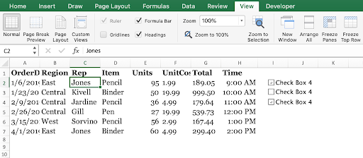
8. Add checkboxes to your spreadsheet

Add an interactive checkbox to Excel spreadsheets
Did you know that you can add checkboxes to your Excel spreadsheets? Now you do. Here’s how to do it. Make sure that your Developer tab is enabled in the Ribbon!
- Highlight the cell you want to add a checkbox to.
- Switch to the Developer tab in the Ribbon.
- Add a checkbox or option button depending on what you need in your sheet.
9. Utilize Excel shortcuts
Excel always gets the credit it deserves for providing a large array of features and capabilities to its users. To truly become an expert in Excel, you need to know about keyboard shortcuts. Here are some of the top, most used Excel shortcuts you need to know in order to level up your Excel game right now:
- Select a column: Click on a cell in a column, then press the Ctrl + Space keys.
- Select a row: Click on a cell in a row, then press the Shift + Space keys.
- Start a new line in a cell: Press Alt + Enter as you type to start a new line.
- Insert current time: Press the Ctrl + Shift + Colon ( ; ) keys.
- Insert current date: Press Ctrl + Colon ( ; ) keys.
- Hide a column: Press the Ctrl + 0 keys.
- Hide a row: Press the Ctrl + 9 keys.
- Show or hide formulas: Press the Ctrl + Tilde ( ~ ) keys.
10. Remove gridlines from a spreadsheet
If you want a completely blank canvas in Excel, you can remove the grid lines from any spreadsheet in one single click. Go to the View tab in the Ribbon, then deselect the Gridlines option in the Show section.
11. Quickly insert a Pivot Table
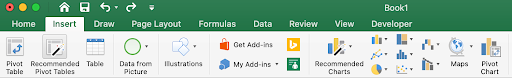
Pivot Tables are extremely useful when analyzing and presenting your data. Select all of the cells you want to use, then create a Pivot Table by going to the Insert tab and clicking Recommended Pivot Tables.
12. Add comments to your formulas
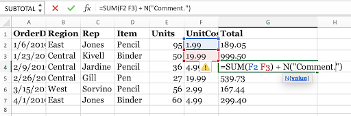
Comments are an easy way to search your formulas or make them more understandable for viewers. To add a comment, simply add + N(“Comment here”) after your formula. This won’t show up in the cell itself, however, you’ll be able to see it in the formula bar.
13. Draw your equations
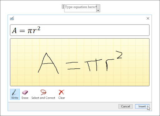
Excel converts your handwritten equations to text (Source: HowToGeek)
In Excel 2016 and later, you’re able to draw equations and have Excel convert them into text.
- Go to the Insert tab in the Ribbon.
- Click on Equation, then select Ink Equation.
- Write your equation inside the yellow box.
Final thoughts
If you’re looking for other guides or want to read more tech-related articles, consider subscribing to our newsletter. We regularly publish tutorials, news articles, and guides to help you.
You May Also Like:
> How to Reference Another Sheet in Excel
> How to Create Excel Header Row
> Top 51 Excel Templates to Boost Your Productivity