


INDEX/MATCH is a powerful alternative to Excel VLOOKUP, allowing users to perform advanced searches with multiple criteria. This method offers more flexibility and speed, making it a preferred option for many users.
This tutorial will guide you through the steps to replace VLOOKUP with INDEX/MATCH in Excel. You will learn how to set up the INDEX/MATCH formula, use it to retrieve data and troubleshoot common errors.
By the end of this article, you can replace VLOOKUP with INDEX/MATCH, allowing you to work more efficiently and effectively in Excel. Let's get started!
Table of Contents
- Excel INDEX and MATCH Basics
- INDEX MATCH vs. VLOOKUP: Which One to Use in Excel?
- 4 Reasons Why INDEX MATCH is Better Than VLOOKUP
- Using INDEX MATCH in Excel
- Using Excel INDEX MATCH with Functions
- FAQs
- Final Thoughts
Excel INDEX and MATCH Basics
This tutorial is about how to use INDEX and MATCH functions in Excel to do a VLOOKUP. The INDEX function returns a value in an array based on the row and column numbers you specify.
Meanwhile, the MATCH function searches for a lookup value in a range of cells and returns the relative position of that value in the range.
To use these functions together, you need to use the MATCH function to determine the row and column numbers of the data you want to retrieve and then use the INDEX function to retrieve that data.
To use the INDEX function, specify the range of cells from which you want to return a value, the row number, and the column number. If you omit one of the numbers, the other is required.
Here's an example table that we can use to demonstrate how to use the INDEX and MATCH functions together:
Let's say you want to retrieve the price of bananas. Instead of using VLOOKUP, you can use the INDEX and MATCH functions together.
First, you would use the MATCH function to determine the row number of "Banana" in the "Fruit" column:
=MATCH("Banana", A2:A5, 0)
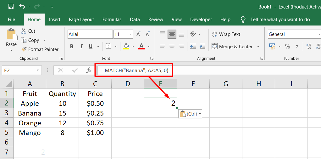
This formula will return the value "2", since "Banana" is in the second row of the "Fruit" column.
Next, you would use the MATCH function again to determine the column number of "Price" in the header row:
=MATCH("Price", A1:C1, 0)
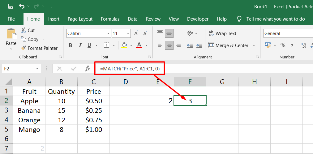
This formula will return the value "3", since "Price" is in the third column of the header row.
Finally, you can use the INDEX function to retrieve the price of bananas from the table:
=INDEX(A1:C5, 2, 3)
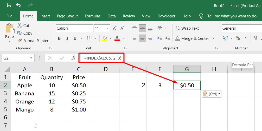
This formula will return the value "$0.50", the price of bananas.
Using these two functions together can be very helpful when working with real data. It allows you to retrieve data based on specific criteria rather than just looking up values in a table.
Combining INDEX and MATCH allows you to create more complex lookup formulas and perform advanced searches with multiple criteria.
INDEX MATCH vs. VLOOKUP: Which One to Use in Excel?
When looking for information in Excel, different functions can be used. Two popular ones are VLOOKUP and INDEX MATCH. Although VLOOKUP is simpler, INDEX MATCH has more benefits.
Here are some reasons why INDEX MATCH is better:
- Flexibility: With VLOOKUP, the lookup value must be in the first column of the table. With INDEX MATCH, you can look up values in any column, making it more flexible.
- Accuracy: VLOOKUP only searches for exact matches, while INDEX MATCH can also handle approximate matches. If your data is not exact, INDEX MATCH can still find the closest match.
- Speed: INDEX MATCH is faster than VLOOKUP when searching large amounts of data. VLOOKUP can slow down your spreadsheet when searching through a large table.
- Readability: INDEX MATCH formulas are easier to read and understand than VLOOKUP formulas. This makes it easier for others to understand your formulas if they need to work with your spreadsheet.
While VLOOKUP may be simpler, INDEX MATCH is more flexible, accurate, faster, and easier to read. So, it's worth taking the time to learn how to use it.
4 Reasons Why INDEX MATCH is Better Than VLOOKUP
- Right to left lookup: VLOOKUP can only search for values to the right of the lookup column, but INDEX MATCH can look up values to the left. This is helpful when your lookup value is outside the leftmost column of the table.
- Safe insert or delete of columns: When using VLOOKUP, adding or deleting columns can break your formula because you have to specify the column index. With INDEX MATCH, you specify the return column range, so you can add or delete columns without changing the formula.
- No limit for lookup value size: VLOOKUP has a limit of 255 characters for the lookup value, but INDEX MATCH can handle long strings in your data.
- Faster processing speed: If you have large data sets, INDEX MATCH will be faster than VLOOKUP because it only processes the lookup and returns columns, not the entire table. This is especially important if your workbook has many complex formulas.
If you want to make your Excel formulas more flexible, accurate, and efficient, consider using INDEX MATCH instead of VLOOKUP.
Using INDEX MATCH in Excel
Let's say we have a table of fruits and their prices, but we want to know the price of a specific fruit, even though the fruit names are in the second column of the table. We can use the INDEX MATCH function to find the price of the fruit we're looking for.
First, we would select the cell where we want the result to appear. Then, we would type in the following formula:
=INDEX(C2:C8,MATCH("Apple",B2:B8,0))
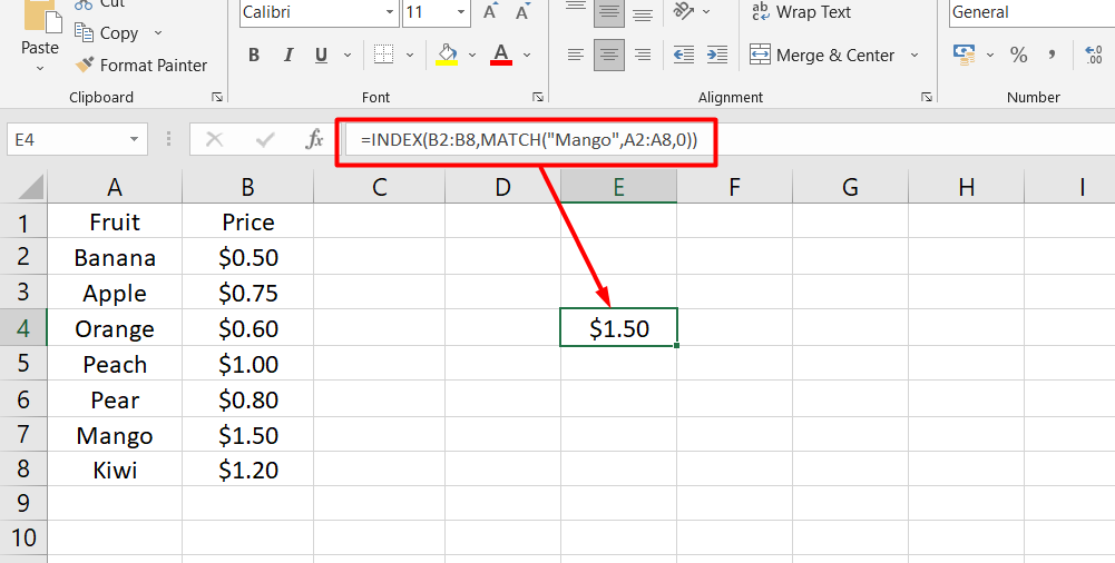
Here's what that formula means:
INDEX(C2:C8) tells Excel to look for the result in the price column (column C).
MATCH("Apple",B2:B8,0) tells Excel to find the row where the fruit name "Apple" is located in the table (which is in column B). The "0" at the MATCH function's end means we want an exact match.
Putting it all together, the formula tells Excel to look in the price column for the row where "Apple" is located and return the corresponding price.
Using the INDEX MATCH function, we can easily look up information in Excel, even if our lookup value isn't in the leftmost column of our table.
Using Excel INDEX MATCH with Functions
In Excel, you can use functions like MAX, MIN, and AVERAGE to find the largest, smallest, and average values in a range of data. But what if you need to get a value from another column corresponding to those values? That's where INDEX MATCH comes in handy.
Let's say we have a table of fruits, their prices, and their sales numbers. We want to find the fruit with the highest sales and get its price. We can do it using the INDEX MATCH with MAX formula:
- Select the cell where you want the result to appear.
- Type in the following formula: =INDEX(B2:B8, MATCH(MAX(C2:C8), D2:D8, 0))
Here's what that formula means:
- INDEX(B2:B8) tells Excel to look for the result in the price column (column B).
- MATCH(MAX(C2:C8), D2:D8, 0) tells Excel to find the row where the largest sales number is located in the table (which is in column D). The "0" at the MATCH function's end means we want an exact match.
- Putting it all together, the formula tells Excel to look in the price column for the row where the highest sales number is located and return the corresponding price.
By using the INDEX MATCH with MAX, we can easily find the price of the fruit with the highest sales.
You can use similar formulas to find the smallest value with INDEX MATCH with MIN and the value closest to the average with INDEX MATCH with AVERAGE. Adjust the match_type argument in the MATCH function depending on how your data is organized.
Here's a table to illustrate the example:
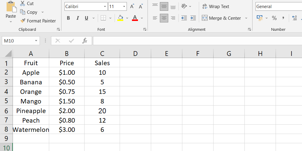
By using INDEX MATCH with MAX, we can find that the fruit with the highest sales is Pineapple, which is $2.00.
FAQs
Is INDEX MATCH better than VLOOKUP?
INDEX MATCH is often considered more flexible and powerful than VLOOKUP because it allows for vertical and horizontal lookups, multiple criteria, and dynamic ranges.
What is the formula to replace VLOOKUP in Excel?
The formula to replace VLOOKUP in Excel is the INDEX MATCH combination, where INDEX returns the value from a specified range based on a matched criterion obtained with MATCH.
How do I use INDEX MATCH in Excel?
To use INDEX MATCH in Excel, you need to specify the range of values you want to search in, use the MATCH function to find the position of the desired value, and then use INDEX to retrieve the corresponding value from another range.
Why use INDEX MATCH in Excel?
INDEX MATCH in Excel offers greater flexibility for performing lookups as it can handle both vertical and horizontal searches, multiple criteria, and allows for more advanced data retrieval compared to VLOOKUP.
How do I match two lists in Excel?
To match two lists in Excel, you can use the MATCH function to find the position of a value in one list and then use INDEX to retrieve the corresponding value from the other list, or you can use the VLOOKUP or INDEX MATCH combination to compare and retrieve matching values.
Final Thoughts
In conclusion, while VLOOKUP is a useful function, INDEX/MATCH is a more powerful and versatile option for looking up information in Excel.
By combining the INDEX and MATCH functions, users can perform left-to-right and right-to-left lookups, and can even perform more complex lookups by nesting functions.
Ultimately, learning to use INDEX/MATCH can save time and increase efficiency when working with data in Excel.
One more thing
If you have a second, please share this article on your socials; someone else may benefit too.
Subscribe to our newsletter and be the first to read our future articles, reviews, and blog post right in your email inbox. We also offer deals, promotions, and updates on our products and share them via email. You won’t miss one.
Related articles
» How to Limit Rows and Columns in an Excel Worksheet
» Troubleshooting "OLE Action Excel" Error in Microsoft Excel
» Ways To Alternate Row Colors in Excel [Guide/]