Excel alternate row color is a simple but effective way to make your data more readable. With Excel alternate row color feature, you can distinguish rows and easily track changes in your data.
Whether you are creating a budget spreadsheet or managing customer information, this feature can help improve the readability of your data.
Following this guide can add a professional touch to your Excel spreadsheets, making them more user-friendly. So, let's learn how to use Excel alternate row color to improve your data visualization.
![Ways To Alternate Row Colors in Excel [Guide]](https://cdn.shopify.com/s/files/1/0090/2125/9831/files/excel_alternate_row_color-1.jpg?v=1705313798)
Jump to Section:
- What are alternating colors in Excel?
- How do I alternate row colors in sheets?
- Use conditional formatting to apply banded rows or columns
- Benefits of using alternating row colors for data visualization
- Tips for choosing colors for alternating rows in Excel
- How to turn off alternating row colors in Excel
- Final Thoughts
What are alternating colors in Excel?
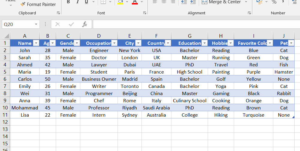
In Microsoft Excel, alternating colors refer to applying a different color to every other row or column in a table or spreadsheet. This technique is also known as color banding. It is a formatting tool that helps users to read and analyze data quickly and easily.
Applying alternating colors to a table helps distinguish each row and column from one another, especially when you have a lot of data. It makes it easier for the reader to track information from left to right and from top to bottom.
For example:
If you have a table with hundreds of rows and columns, it can be difficult to read and understand the data. But if you apply alternating colors to every other row or column, it can help to make the data more comprehensible.
Excel provides an easy way to apply alternating colors to a table or spreadsheet. You can choose from a variety of preset table formats, or you can customize the colors and shading to your liking. Additionally, you can easily turn off the alternating colors feature by unchecking the "Banded rows" option in the Design tab.
A Step-by-Step Guide for Improved Readability with Excel Alternate Row Color
How do I alternate row colors in sheets?
Adding color banding to alternate rows or columns can significantly improve the data readability in your Excel worksheet. Here is a simple step-by-step guide on how to format alternate rows or columns in Excel:
- Select the range of cells that you want to format.
- Click on the "Home" tab in the ribbon.
-
Click on the "Format as Table" option. A list of table styles will appear.
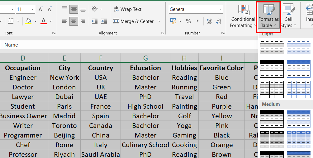
- Pick a table style that has alternate row or column shading. Excel will automatically apply the shading to the selected range of cells.
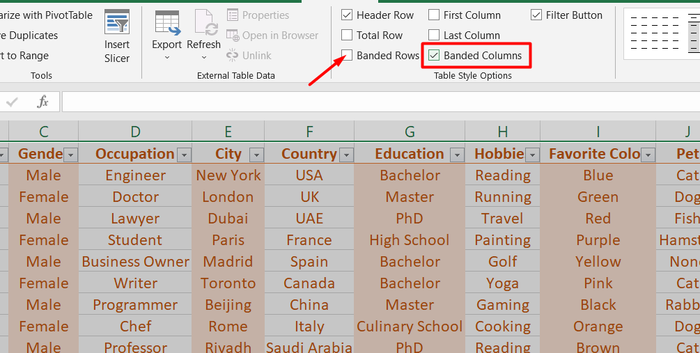
- To change the shading from rows to columns, select the table, click on the "Design" tab, and uncheck the "Banded Rows" box.
-
Check the "Banded Columns" box.
Note:
You can convert the table to a data range if you want to keep the banded table style without the table functionality. Although color banding won't continue automatically, you can copy alternate color formats to new rows using the "Format Painter" tool.
Following these simple steps, you can quickly and easily format alternate rows or columns in Excel, making scanning and analyzing your data easier.
Use conditional formatting to apply banded rows or columns
Formatting your Excel worksheet with alternating row colors can make it easier to read and understand. You can achieve this effect by applying a preset table format, or by using a conditional formatting rule to apply different formatting to specific rows or columns. Here's how to use the conditional formatting option:
- Select the range of cells you want to format or click the Select All button to apply the formatting to the entire worksheet.
-
Click the Home tab, then click the Conditional Formatting dropdown and select New Rule.
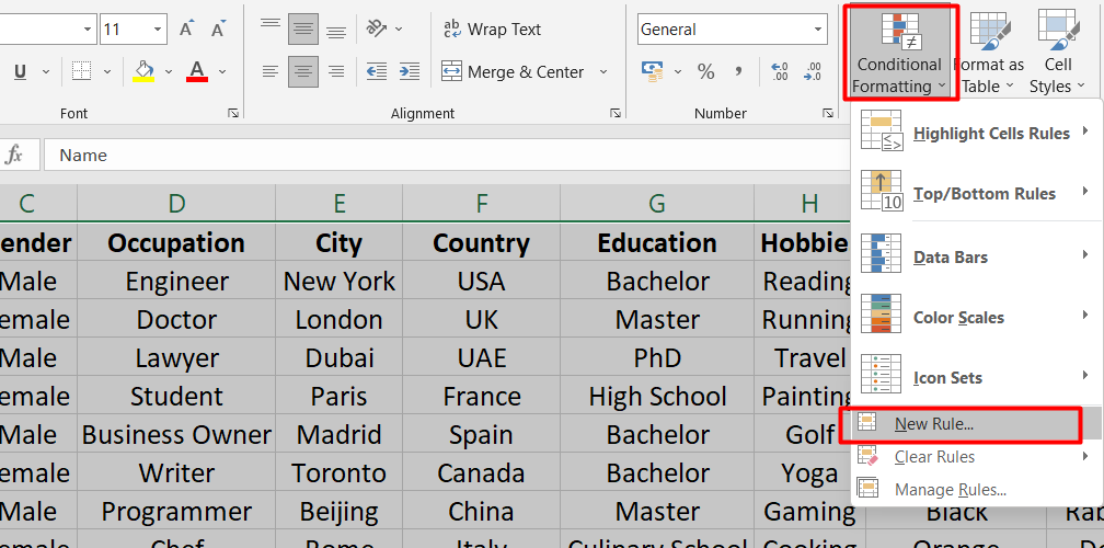
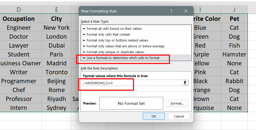
- In the New Formatting Rule dialog box, select "Use a formula to determine which cells to format" in the "Select a Rule Type" box.
-
To apply color to alternate rows, type the formula =MOD(ROW(),2)=0 in the "Format values where this formula is true" box. To apply color to alternate columns, use this formula: =MOD(COLUMN(),2)=0.
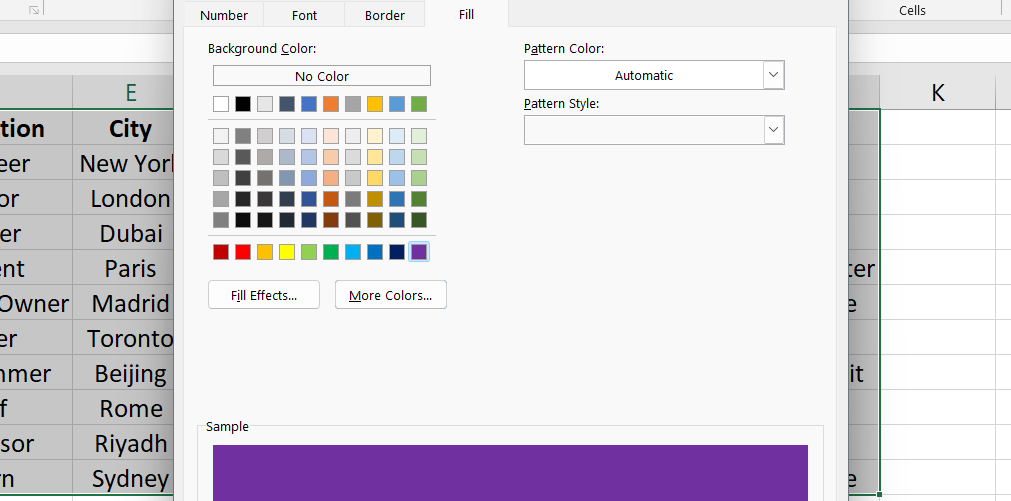
-
Click the "Format" button, select "Fill" and pick a color to use for your alternating rows or columns.
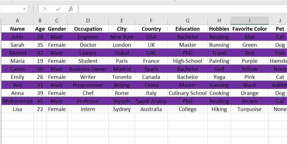
-
Click "OK" to close all the dialog boxes and see your new formatting.
Some tips to remember:
- To edit the conditional formatting rule, select one of the cells that has the rule applied, then click Home > Conditional Formatting > Manage Rules > Edit Rule and make your changes.
- To clear conditional formatting from cells, select them, click Home > Clear, and pick Clear Formats.
- To copy the conditional formatting to other cells, select one of the cells that has the rule applied, click Home > Format Painter button, and then click the cells you want to format.
Benefits of using alternating row colors for data visualization
Using alternating row colors or color banding is a helpful way to make data in your spreadsheet easier to read. Color banding adds color to every other row or column in your spreadsheet, making it easy for your eyes to follow along with the information.
You can apply color banding by selecting a range of cells and choosing a table style that has alternate row shading. If you want to keep the table style without the table functionality, you can convert the table to a data range.
Alternating row or column shading is automatically applied when you add more rows or columns. This technique is particularly useful when working with large amounts of data, as it allows you to quickly and easily differentiate between rows or columns.
Tips for choosing colors for alternating rows in Excel
When choosing colors for alternating rows in Excel, there are a few tips you can follow to make sure your data is easy to read and looks good:
- Use colors that are easy on the eyes: Avoid using colors that are too bright or hard to read. Choose colors that are easy to distinguish from one another.
- Stick with a simple color scheme: Too many colors can make your data look cluttered and confusing. Stick to a simple color scheme, such as two or three colors that complement each other.
- Use colors that match your branding: If you're using Excel to create a report or presentation, you may want to use colors that match your company's branding. This can help your data look more professional and consistent with other materials.
- Consider colorblindness: About 8% of men and 0.5% of women have some form of color blindness, so choosing colors that are easy to distinguish for those with color vision deficiencies is important.
By following these tips, you can choose colors for alternating rows in Excel that make your data easy to read and look great.
How to turn off alternating row colors in Excel
Here's a list of steps on how to turn off alternating row colors in Excel:
- Open the Excel worksheet that contains the table with alternating row colors.
- Click on any cell within the table to select it.
- Go to the Design tab, located at the top of the screen.
- Look for the "Table Styles" section on the Design tab and find the "Banded Rows" option.
-
Uncheck the "Banded Rows" option by clicking on the checkbox next to it.
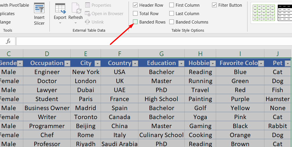
- The alternating row colors will be turned off immediately.
- Save your changes by clicking on the Save button at the top of the screen.
By following these steps, you can easily turn off alternating row colors in Excel.
Final Thoughts
In conclusion, alternating row colors is a great way to make your Excel table easier to read and navigate. This feature lets you quickly identify and track specific data in your worksheet.
There are several ways to apply alternating row colors, such as using built-in table styles, using conditional formatting, or manually formatting the cells. When choosing colors for your table, it is important to consider accessibility and legibility and to use a color scheme that matches your purpose and audience.
Finally, if you no longer want to use alternating row colors, you can turn off this feature by unchecking the Banded Rows option in the Design tab.
One more thing
We’re glad you've read this article upto here :) Thank you for reading.
If you have a second, please share this article on your socials; someone else may benefit too.
Subscribe to our newsletter and be the first to read our future articles, reviews, and blog post right in your email inbox. We also offer deals, promotions, and updates on our products and share them via email. You won’t miss one.
Related articles
» How To Use NOW Function In Excel To Get Current Date And Time
» How to Merge Multiple Tables in Excel for Better Data Management
» How to use the EDATE function in Excel