How to Calculate Break-Even Analysis in Excel

Excel has many functions. Other than the normal tabulations, Excel can help you in various business calculations, among other things being Break-Even analysis.

Table of Contents

• How to calculate Break-even analysis in Excel
• What is break-even analysis
• Break-Even Analysis Formula 
• Contribution Margin 
• Break-Even Point Formula in Excel
• Calculate break-even analysis with Goal-Seek
• Calculate Break-Even analysis in Excel with formula
• Calculate Break-Even analysis with chart

How to calculate Break-even analysis in Excel

Break-even analysis is the study of what amount of sales or units sold, a business requires to meet all its expenses without considering the profits or losses. It occurs after incorporating all fixed and variable costs of running the operations of the business.

In this post, we focus on how to use Excel to calculate Break-Even analysis. 

What is break-even analysis

The break-even point of a business is where the volume of production and volume of sales of goods (or services) sales are equal. At this point, the business can cover all its costs. In the economic sense, the break-even point is the point of an indicator of a critical situation when profits and losses are zero. Usually, this indicator is expressed in quantitative or monetary units.

The lower the break-even point, the higher the financial stability and solvency of the firm.

Break-even analysis is critical in business planning and corporate finance because assumptions about costs and potential sales determine if a company (or project) is on track to profitability.

Break-even analysis helps organizations/companies determine how many units they need to sell before they can cover their variable costs and the portion of their fixed costs involved in producing that unit.

Break-Even Analysis Formula 

To find the break-even, you need to know:

• Fixed costs 
• Variable costs
• Selling price per unit
• Revenue 

The break-even point occurs when:

Total Fixed Costs (TFC) + Total Variable Costs (TVC) = Revenue

• Total Fixed Costs are known items such as rent, salaries, utilities, interest expense, amortization, and depreciation. 
• Total Variable Costs include things like direct material, commissions, billable labour, and fees, etc.
• Revenue is Unit Price * Number of units sold.

Contribution Margin 

A key component of calculating the break-even analysis is understanding how much margin or profit is generated from sales after subtracting the variable costs to produce the units. This is called a contribution margin. Thus: 

Contribution Marin =  Selling Price - Variable Costs 

Break-Even Point Formula in Excel

You can calculate the break-even point with regard to two things:

1. Monetary equivalent: (revenue*fixed costs) / (revenue - variable costs).
2. Natural units: fixed cost / (price - average variable costs).

Bearing this in mind, there are a number of ways to calculate the break-even point in Excel:

1. Calculate break-even analysis with Goal-Seek Feature (a built-in Excel tool)
2. Calculate break-even analysis with a formula
3. Calculate break-even analysis with a chart

Calculate break-even analysis with Goal-Seek

Case: Supposing you want to sale a new product. You already know the per unit variable cost and the total fixed cost. You want to forecast the possible sales volumes, and use this to price the product. Here is what you need to do.

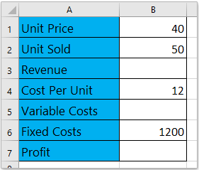
1. Make an easy table, and fill in items/data.
   
   
   
   
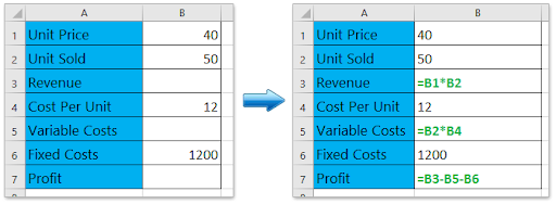
2. In Excel, enter proper formulas to calculate the revenue, the variable cost, and profit. 
   1. Revenue = Unit Price x Unit Sold
   2. Variable Costs = Cost per Unit x Unit Sold
   3. Profit = Revenue – Variable Cost – Fixed Cost 
   4. Use these formulas for your calculation.
      
      
      
      
      
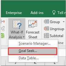
3. On your Excel document, Click the Data > What-If Analysis > select Goal Seek.
   
   
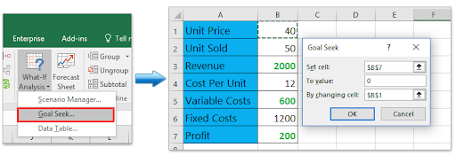
4. When you open the Goal Seek dialogue box, do as follows:
   1. Specify the Set Cell as the Profit cell; in this case, it is Cell B7;
   2. Specify the To value as 0;
   3. Specify the By changing cell as the Unit Price cell, in this case; it is Cell B1.
   4. Click the OK button
      
5. The Goal Seek Status dialogue box will pop up. Please click the OK to apply it.
   
   
   
   

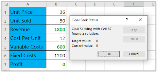
Goal Seek will change the Unit Price from 40 to 31.579, and the net profit changes to 0. Remember, at break-even point profit is 0. Therefore, if you forecast the sales volume at 50, the Unit price cannot be less than 31.579. Otherwise, you will incur a loss.

Calculate Break-Even analysis in Excel with formula

You can also calculate the break-even on point on Excel using the formula. Here’s how:

1. Make an easy table, and fill items/data. In this scenario, we assume we know the units sold, cost per unit, fixed cost, and profit.
   
   
   
   
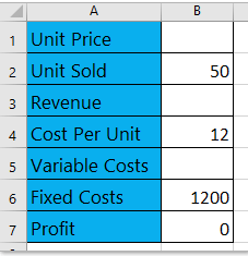
2. Use the formula for calculating the missing items/data.
1. Type the formula = B6/B2+B4 into Cell B1 to calculating the Unit Price, 
2. Type the formula = B1*B2 into Cell B3 to calculate the revenue,
3. Type the formula = B2*B4 into Cell B5 to calculate variable costs. 

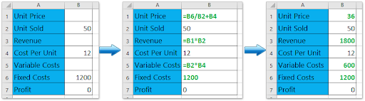
Note: if you change any value, for instance, the value of the forecasted unit sold or cost per unit or fixed costs, the value of the unit price will change automatically. 

Calculate Break-Even analysis with chart

If you have already recorded your sales data, you can calculate the break-even point with a chart in Excel. Here’s how:

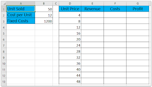
1. Prepare a sales table. In this case, we assume we already know the sold units, cost per unit, and fixed costs, and we assume they’re fixed. We need to make the break-even analysis by unit price.
   
   
2. Finish the calculations of the table using the formula
   
   
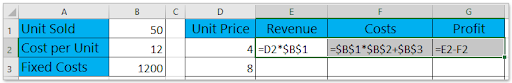
   1. In the Cell E2, type the formula =D2*$B$1 then drag its AutoFill Handle down to Range E2: E13;
   2. In the Cell F2, type the formula =D2*$B$1+$B$3, then drag its AutoFill Handle down to Range F2: F13;
   3. In the Cell G2, type the formula =E2-F2, then drag its AutoFill Handle down to the Range G2: G13.
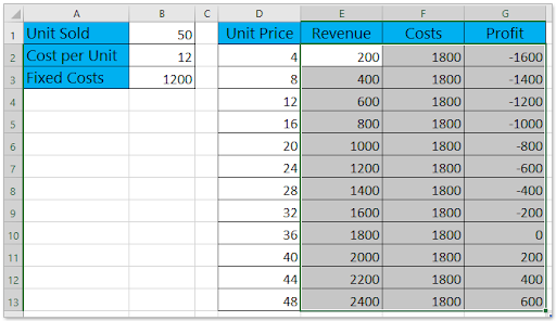
3. This calculation should give you the source data of the break-even chart.
   
   
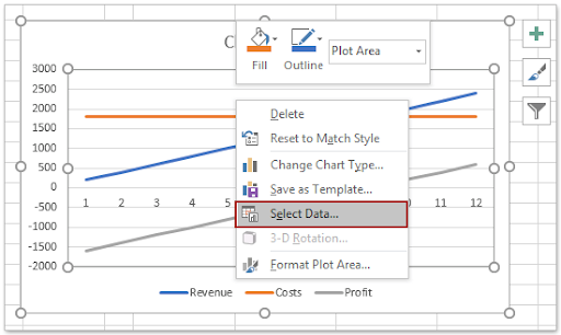
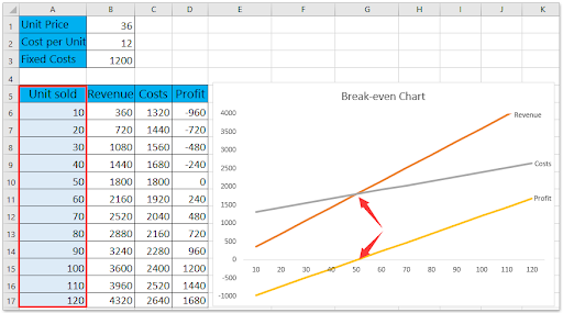
4. On the Excel table, select the Revenue column, Costs column, and Profit column simultaneously, and then click Insert > Insert Line or Area Chart > Line. This will create a line chart.
   
   
   
   
5. Next, right-click the chart. From the context menu, click Select Data.
   
   
   
   
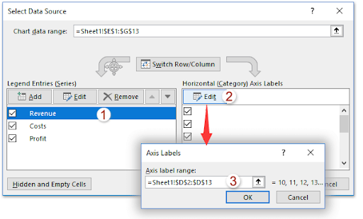
6. In the Select Data Source dialogue box, do the following:
1. In the Legend Entries (Series) section, select one of the series as you need. In this case, we select the Revenue series;
2. Click the Edit button in the Horizontal (Category) Axis Labels section;
3. A dialogue box will pop out with the name Axis Labels. In the box specify the Unit Price column (except the column name) as axis label range;
4. Click OK > OK to save the changes.
   
   
7. A chat will be created, called the break-even chart. You will notice the break-even point, which occurs when the price equals to 36.
   
   
8. Similarly, you can create a break-even chart to analyze the break-even point by sold units:
   

You’re done. Its that simple. 

Wrapping up 

You can tweak the appearance of your data through the data section and design tools. Excel allows you to do many other things with the data. 

If you’re looking for more guides or want to read more tech-related articles, consider subscribing to our newsletter. We regularly publish tutorials, news articles, and guides to help you.