
Excel Conditional Formatting is a powerful tool that helps you highlight specific data based on certain conditions. This feature lets you easily identify trends, analyze data, and make informed decisions. This easy tutorial will show you how to use Excel's Conditional Formatting to its full potential.
Whether you're a beginner or an experienced user, this tutorial will provide step-by-step instructions and practical examples. By the end of this article, you will be able to apply different formatting styles to your data based on criteria such as cell values, dates, or text.
Trust us to guide you through this process and help you enhance your data visualization skills. Let's dive in and explore the possibilities of Excel Conditional Formatting.
Table of Contents
- Understanding Conditional Formatting
- Highlighting Cells Based on Criteria
- Applying Formatting to Cells with Data Bars
- Creating Color Scales and Icon Sets
- Using Conditional Formatting with Dates
- Applying Formatting to Top or Bottom-Ranked Values
- FAQs
- Final Thoughts
Understanding Conditional Formatting
Conditional formatting is a great tool in Microsoft Excel that helps you highlight specific values or cells that meet certain criteria. It is like having a magic wand that can change the appearance of your cells based on a specific condition you set.
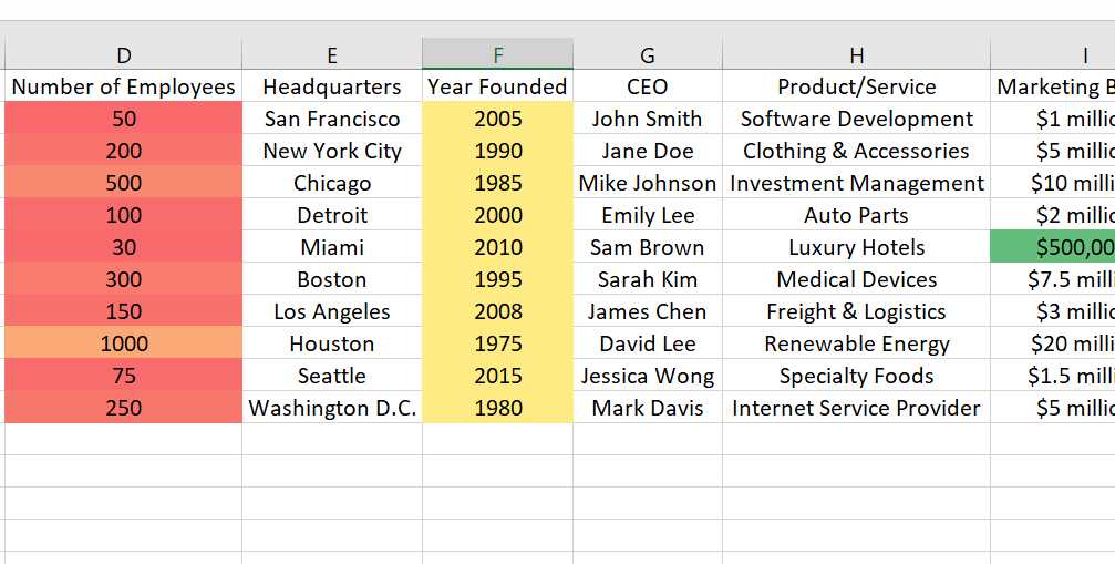
For example, let's say you want to identify all the cells in your table that contain numbers greater than 50. You can easily use conditional formatting to change the color or font of those cells to make them stand out from the rest. This makes it easy to identify and analyze data.
There are many different ways to use conditional formatting in Excel. You can use it to highlight cells based on their values, format cells based on specific dates, or identify duplicate or unique values in a range of cells. You can customize the formatting style using different color scales, data bars, and icon sets.
Conditional formatting is a powerful tool that can help you quickly and easily identify important information in your Excel spreadsheets.
Highlighting Cells Based on Criteria
Excel's conditional formatting can help you do just that. One way to use this feature is by highlighting cells based on specific criteria.
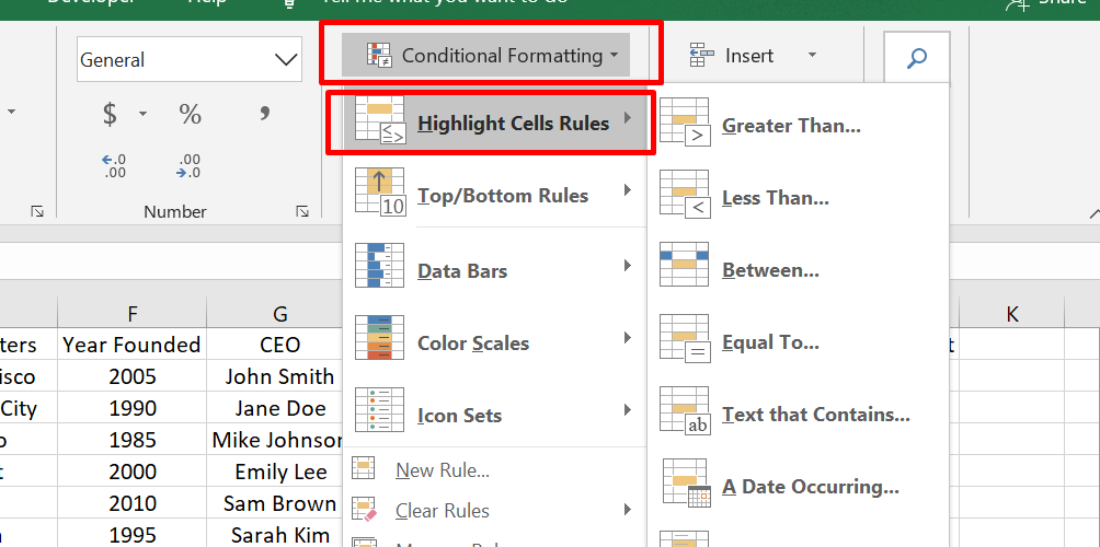
- Select the range of cells, tables, or entire sheets to which you want to apply the formatting.
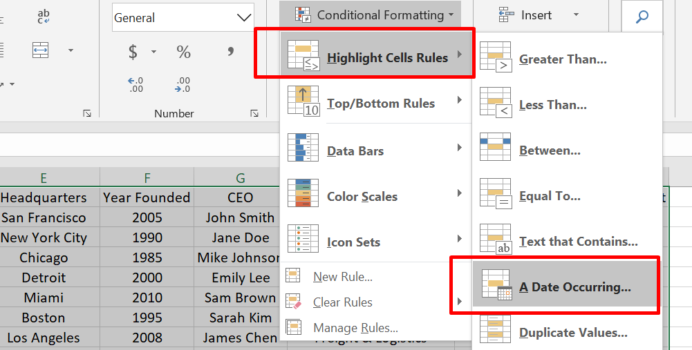
- Go to the Home tab and click on the Conditional Formatting option.
- Choose different Highlight Cell Rules, such as Text that Contains.
Let's say you want to find all cells that contain the word "apple" in a list of fruits. Type "apple" in the box next to "containing" and click OK. This will highlight all cells that contain the word "apple" in the selected range.
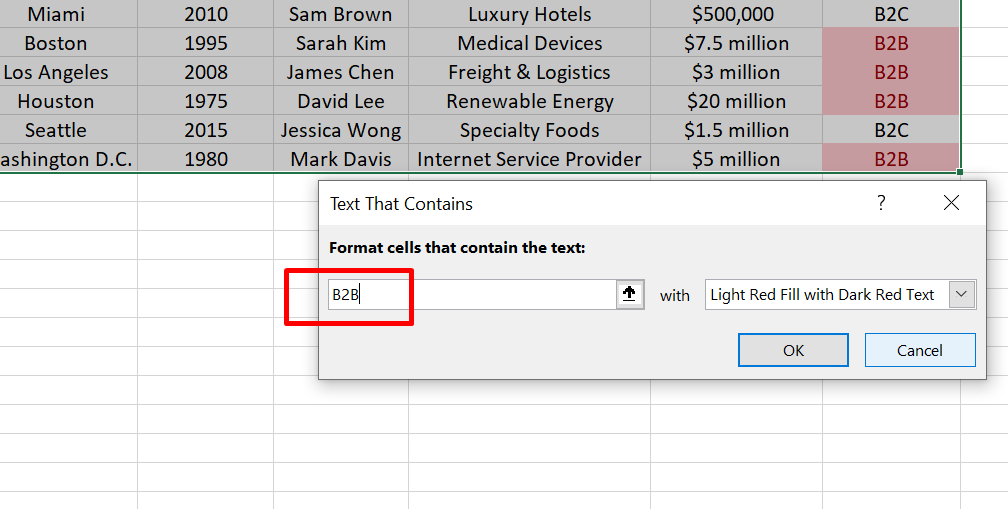
You can also use other criteria to highlight cells, such as those containing specific values, dates, or formulas. Conditional formatting makes it easy to identify specific information in a large table quickly and can help you save time and make more informed decisions.
Applying Formatting to Cells with Data Bars
Conditional formatting is a great feature in Microsoft Excel that can help you visually represent data meaningfully. One way to do this is by applying formatting to cells with data bars.
- Select the range of cells, tables, or entire sheets to which you want to apply the formatting.
- Go to the Home tab
- Under Format, click on Conditional Formatting
- Point to Data Bars, and choose a gradient or solid fill
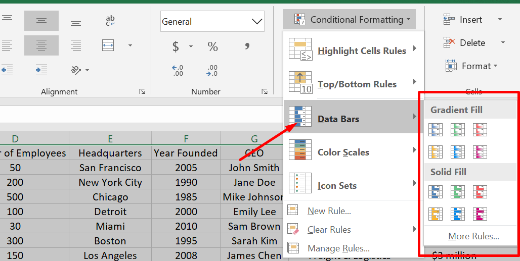
Data bars are horizontal bars placed behind the cell's data to represent its value. For example, if you have a list of sales figures, you can use data bars to quickly visualize which numbers are higher or lower. The longer the data bar, the higher the value of the cell.
You can customize the look of the data bars by changing the color, gradient, or border style. This makes it easy to highlight specific information and create professional-looking spreadsheets.
Data bars are a powerful tool in Excel that can help you quickly understand and analyze data. Whether you're a student, teacher, or business professional, this feature can help you make more informed decisions based on the data you have.
Creating Color Scales and Icon Sets
Conditional formatting is a useful feature in Microsoft Excel that can help you make sense of data by visually representing it differently. One way to do this is by using color scales and icon sets.
- Select the range of cells that you want to format. This could be a table or a specific area of your worksheet
- Go to the Home tab and click on Conditional Formatting in the Styles group.
- Point to Color Scales and choose the type of color scale that you want to use.
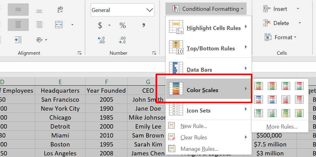
Color scales are a way to visually represent the value of a cell based on its color. For example, you might choose a green-yellow-red color scale to represent the value of sales figures. The cells with the highest sales numbers would be colored green, the cells with average sales figures would be yellow, and the cells with the lowest sales numbers would be red.
Icon sets are another way to represent data visually. They use icons or symbols to represent different values, such as arrows pointing up or down to represent increases or decreases in sales. You can choose from various icon sets to find the one that best suits your needs.
Color scales and icon sets are powerful tools that can help you quickly understand and analyze data in Excel. Whether you're a student, teacher, or business professional, these features can help you make more informed decisions based on the data you have.
Using Conditional Formatting with Dates
Microsoft Excel has a feature called Conditional Formatting that can be used to make it easier to work with dates. This feature can help you quickly identify dates that fall within a certain range or meet specific criteria.
- Select the range of cells that contain the dates you want to work with to use Conditional Formatting with dates.
- Go to the Home tab and click on Conditional Formatting
-
Select Highlight Cell Rules and choose A Date Occurring
- Select one of the date options from the drop-down list in the left-hand part of the window
- Choose from various options, such as dates that occurred last week, this month, or next month.
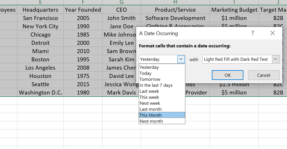
Once you have selected the date range you want to work with, you can choose the formatting you want to apply to the cells. For example, you might highlight the cells in a specific color or add an icon to indicate that the date meets certain criteria.
Conditional Formatting with dates is a useful tool that can help you quickly identify and work with specific dates in Excel. By applying formatting to the cells, you can make it easier to work with and analyze large data sets that include dates.
Applying Formatting to Top or Bottom-Ranked Values
In Microsoft Excel, you can use Conditional Formatting to highlight the top or bottom-ranked values in a range of cells, tables, or PivotTable reports. This can be a useful way to identify trends, outliers, or key data points in a dataset.
- Select one or more cells in the range you want to work with to apply formatting to the top or bottom-ranked values
- Go to the Home tab and find the Styles group
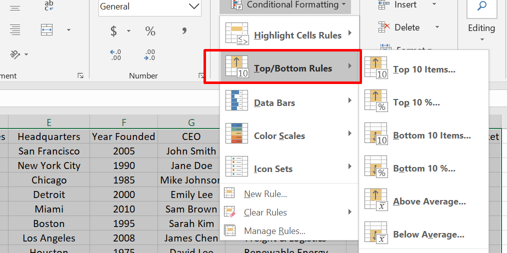
- Click on the arrow next to Conditional Formatting and select Top/Bottom Rules.
-
Choose the command you want to apply, such as Top 10 items or Bottom 10%. You can then enter the values you want to use, such as the number of items to include or the percentage of values you want to highlight.
- Select a format for the top or bottom-ranked values. This can include choosing a color or applying a data bar or icon to the cells.
Applying to format to top or bottom-ranked values is a quick and easy way to highlight key data points in Excel. It can help you identify trends, outliers, and other important information in large datasets.
Excel Conditional Formatting [2021]: All You Need to Know
FAQs
What are the types of conditional formatting in Excel?
The types of conditional formatting in Excel include data bars, color scales, icon sets, cell value rules, and formula-based rules, allowing you to format cells based on specific conditions or criteria.
How do I make Excel automatically change cell color?
To make Excel automatically change cell color, you can use conditional formatting by selecting the cells you want to format, going to the "Home" tab, clicking on "Conditional Formatting," and choosing the desired formatting rule.
How do you change the color of a cell based on value?
To change the color of a cell based on its value, you can apply conditional formatting using the "Highlight Cells Rules" option under the "Conditional Formatting" menu. Select the rule that suits your criteria, such as "Greater Than" or "Less Than," and specify the value and color.
Can you use an if statement to color a cell in Excel?
Yes, you can use an IF statement in Excel to conditionally format a cell by defining the desired formatting within the IF function's true or false arguments based on a specific condition.
How to make cell change color based on positive and negative?
To make a cell change color based on positive and negative values, select the cells you want to format, go to the "Conditional Formatting" menu, choose "Highlight Cells Rules," and select "Greater Than" for positive values and "Less Than" for negative values, specifying the desired colors for each.
Final Thoughts
In conclusion, conditional formatting is a useful tool in Microsoft Excel that can help you highlight important data points. There are many different types of conditional formatting that you can use, such as highlighting cells based on their values, applying data bars, or using color scales.
Using conditional formatting effectively makes your Excel spreadsheets more visually appealing and easier to analyze. This can be especially useful when presenting your data to others or when you need to identify key information quickly.
Overall, conditional formatting can help you get the most out of your Excel spreadsheets with just a few simple clicks.
One more thing
If you have a second, please share this article on your socials; someone else may benefit too.
Subscribe to our newsletter and be the first to read our future articles, reviews, and blog post right in your email inbox. We also offer deals, promotions, and updates on our products and share them via email. You won’t miss one.
Related articles
» How to Use Conditional Formatting to Make Your Excel Data Stand Out
»How to insert page break in Excel worksheet
»Expense Record & Tracking Sheet Templates for Excel
»How to Calculate CAGR in Excel