
However, the good news is that most Excel users rely on a handful of functions covering most of their needs. This resource will unveil the top 10 most useful Excel functions for data analysis.
Table of Contents
- IF Function
- SUMIFS function
- COUNTIFS Function
- TRIM function
- CONCATENATE function
- LEFT and RIGHT functions
- VLOOKUP function
- IFERROR function
- VALUE function
- UNIQUE function
- FAQs
- Final Thoughts
IF Function
The IF function in Excel is a powerful tool that allows for automated decision-making within spreadsheets. With the IF function, you can perform different calculations or display different values based on the outcome of a logical test or decision.
Here's how the IF function works: it requires three components - the logical test to perform, the value to return if the test is true, and the value to return if the test is false. The syntax of the IF function is as follows: =IF(logical test, value if true, value if false).
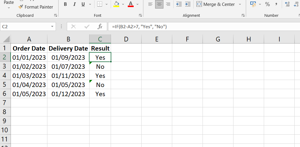
For example, you have a spreadsheet with order dates in column B and delivery dates in column C. You want to display "Yes" if the delivery date is more than 7 days later than the order date and "No" if it is not. In this case, you would use the IF function as follows: =IF(C2-B2>7, "Yes", "No").
This simple IF function formula checks if the delivery date in cell C2 is more than 7 days later than the order date in cell B2. If it is true, it returns "Yes"; otherwise, it returns "No".
SUMIFS function
The SUMIFS function in Excel is an incredibly useful tool for summing values based on multiple criteria. It allows you to specify conditions or criteria to determine which values should be included in the sum.
While Excel also has a function called SUMIF, which can sum values based on a single condition, SUMIFS offers more flexibility as it can test multiple conditions simultaneously. This makes SUMIFS a superior choice when you need to sum values based on multiple criteria.
The syntax of the SUMIFS function is as follows: =SUMIFS(sum range, criteria range 1, criteria 1, ...)
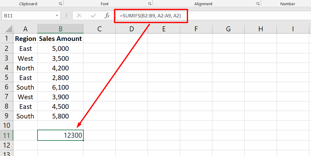
Let's assume the specific region is entered in cell E3 as "East". To calculate the sum of sales amounts for the East region using the SUMIFS function, the formula would be:
=SUMIFS(B2:B9, A2:A9, E3)
In this formula, the sum range is column B (sales amount), the criteria range is column A (region), and the criterion is the value in cell E3 ("East"). The SUMIFS function will sum all the sales amounts that meet the condition of being in the East region.
The result will be the sum of $12,300, representing the total sales amount for the East region based on the given data.
COUNTIFS Function
The COUNTIFS function in Excel is a powerful tool for counting the number of values that meet specific criteria. It works similarly to the SUMIFS function but does not require a sum range.
In addition to COUNTIFS, other similar functions like AVERAGEIFS, MAXIFS, and MINIFS allow you to calculate the average, maximum, and minimum values, respectively, based on multiple criteria.
The syntax of the COUNTIFS function is as follows: =COUNTIFS(criteria range 1, criteria 1, ...)
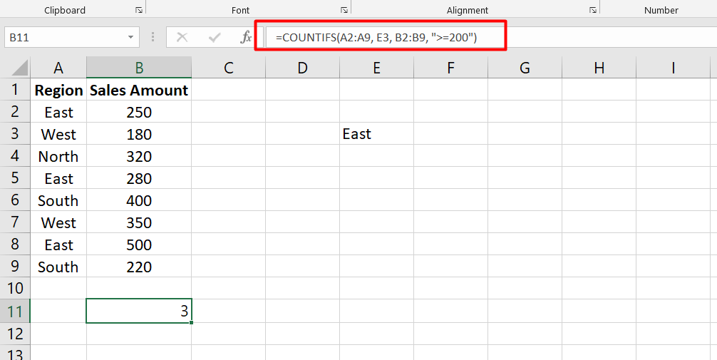
Let's assume the specific region is entered in cell E3 as "East", and we want to count the number of sales from the East region with a value of 200 or more. To calculate this using the COUNTIFS function, the formula would be:
=COUNTIFS(B2:B9, E3, C2:C9, ">=200")
In this formula, the criteria range 1 is column B (region), and the criterion 1 is the value in cell E3 ("East"). The criteria range 2 is column C (sales amount), and the criterion 2 is ">=200". The COUNTIFS function will count the number of sales that meet both conditions.
The result will be the count of 3, indicating that there are three sales in the East region with a value of 200 or more based on the given data.
TRIM function
The TRIM function in Excel is a powerful tool that removes excess spaces from text within a cell, except for the single spaces between words. It is particularly useful for cleaning up data and resolving issues caused by trailing or unnecessary spaces.
One common scenario where TRIM is handy is copying and pasting content from external sources, leading to hidden spaces at the beginning or end of the text. These spaces are not visible to the naked eye but can cause problems when working with the data.
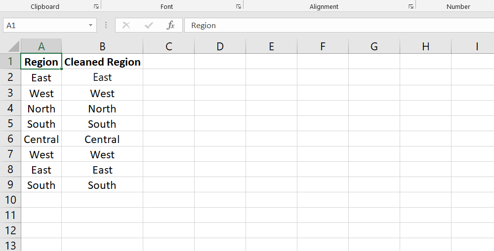
Let's assume there's an accidental space at the end of cell B6, which is causing issues with the COUNTIFS function. To clean up the data and remove any trailing spaces, we can use the TRIM function in a separate column.
In cell C2, you can enter the formula =TRIM(B2), and then drag the formula down to apply it to the remaining cells in column C. The TRIM function will remove any leading or trailing spaces from the region names.
After applying the TRIM function, the modified table will look as follows:
CONCATENATE function
The CONCATENATE function in Excel allows you to combine or concatenate the values from multiple cells into a single cell or text string. It is particularly useful when you merge different parts of text, such as names, addresses, reference numbers, file paths, or URLs.
To use CONCATENATE, you provide the text or cell references you want to join together as arguments within the function. The syntax is as follows: =CONCATENATE(text1, text2, text3, ...).
For example, you have a spreadsheet with first names in column A and last names in column B. You want to create a full name by combining the first and last names with a space in between. In this case, you would use CONCATENATE as follows: =CONCATENATE(A2, " ", B2).
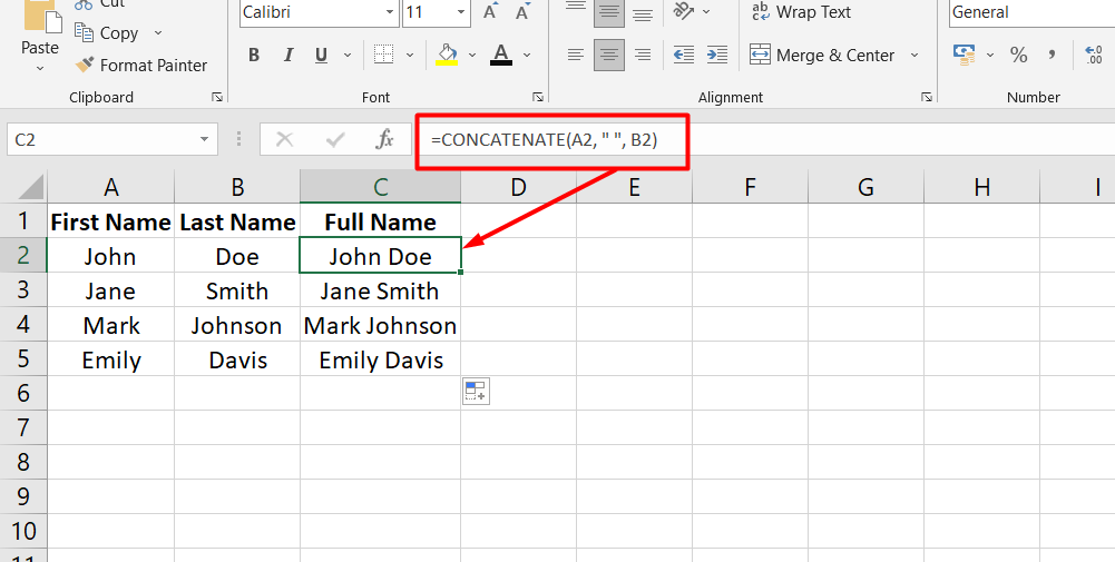
This formula instructs Excel to concatenate the value in cell A2 (the first name), followed by a space, and then the value in cell B2 (the last name). The resulting cell will display the full name.
LEFT and RIGHT functions
The LEFT and RIGHT functions in Excel are useful tools for extracting a specified number of characters from the start or end of a text string, respectively. They offer the opposite action to CONCATENATE and can be utilized to extract specific portions of text, such as parts of an address, URL, or reference, for further analysis.
The LEFT and RIGHT functions require two arguments: the text from which you want to extract characters and the number of characters to be extracted. The syntax for LEFT is =LEFT(text, num chars), while for RIGHT it is =RIGHT(text, num chars).
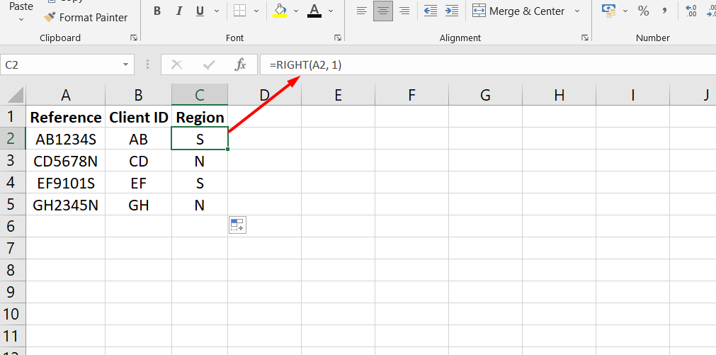
For example, consider a scenario where column A contains references consisting of a client ID (first two characters), a transaction ID, and a region code (final character). To extract the client ID from the references, you would use the LEFT function as follows: =LEFT(A2, 2).
This formula instructs Excel to extract the leftmost two characters from cell A2, representing the client ID. Similarly, the RIGHT function can extract the last character from the cells in column A, indicating whether the client is in the South or the North: =RIGHT(A2, 1).
VLOOKUP function
The VLOOKUP function in Excel is a widely used and essential tool for data analysis. It allows you to search for a value in a table and retrieve information from another column based on that value. This function is particularly valuable for combining data from different lists or comparing two lists for matching or missing items.
To use VLOOKUP, you need to provide four pieces of information:
- The value you want to look for.
- The table in which you want to search.
- The column index number of the column containing the desired information.
- The type of lookup you want to perform (exact match or approximate match).
The syntax for VLOOKUP is as follows: =VLOOKUP(lookup value, table array, column index number, range lookup).
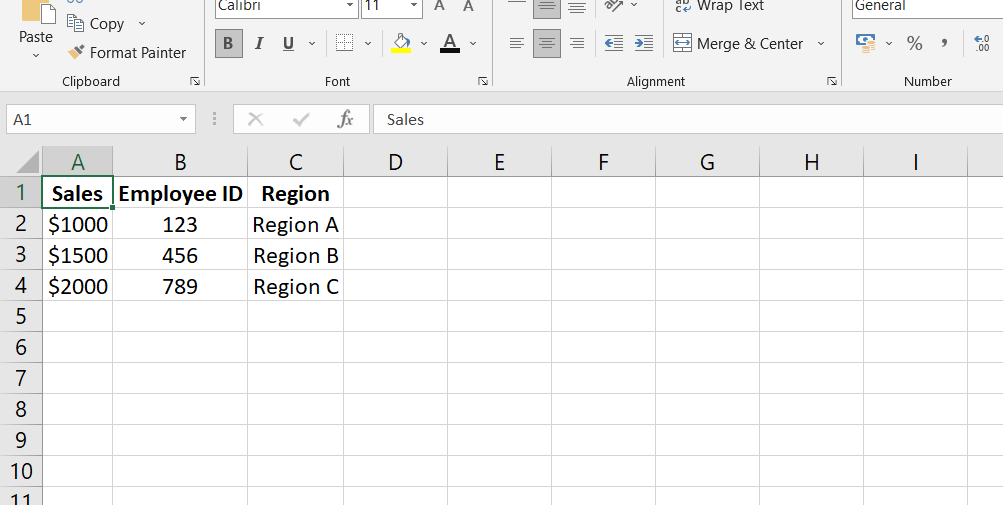
The sales table contains sales amounts in the first column and employee IDs in the second column. We want to bring the corresponding region for each employee from another table into the "Region" column.
Assuming the employee information table is located in cells G2:H12, where column G contains the employee IDs and column H contains the corresponding regions, we can use the VLOOKUP function to retrieve the regions.
In cell C2, you can enter the formula =VLOOKUP(B2, $G$2:$H$12, 2, FALSE). This formula instructs Excel to search for the employee ID in cell B2 within the range $G$2:$H$12. It retrieves the corresponding value from the second column of the range (column H), which represents the region. Copy the formula down to apply it to the remaining cells in the "Region" column.
After applying the VLOOKUP function, the modified table will look as follows:
IFERROR function
The IFERROR function in Excel provides a way to handle and manage errors that may occur in formulas or calculations. It allows you to specify an alternative action or value to display when an error is encountered, providing more meaningful feedback to users and preventing the disruption of data analysis processes.
To use IFERROR, you need to provide two arguments: the value or formula to check for an error and the action or value to perform or display in case of an error.
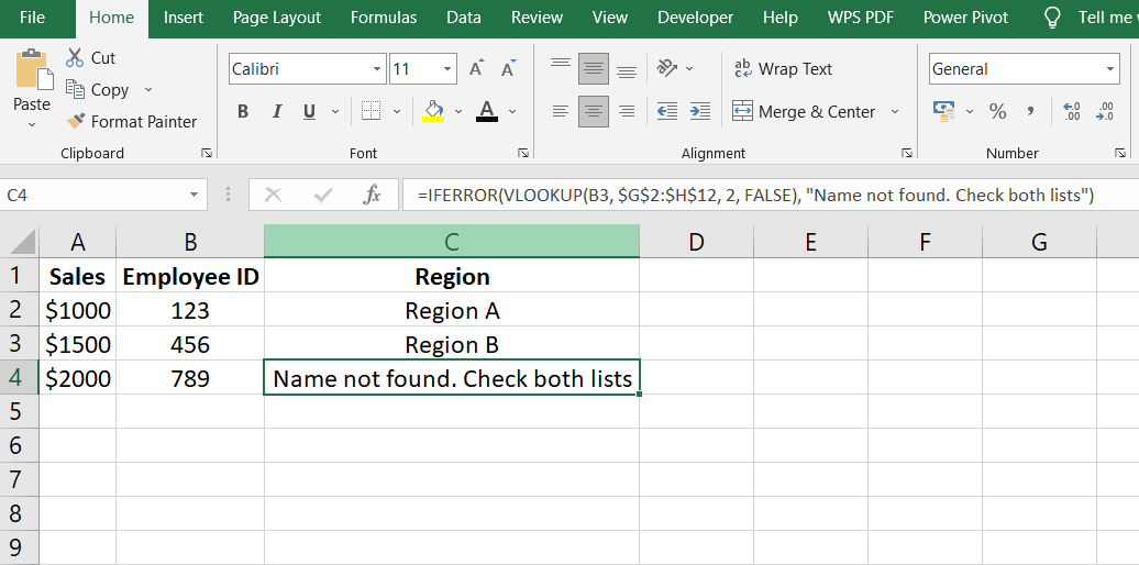
In this table, we have the sales amounts in the first column, employee IDs in the second column, and the corresponding regions in the third column.
Assuming we are using the VLOOKUP function to retrieve the regions based on the employee IDs, we can incorporate the IFERROR function to handle any errors that may occur.
In cell C3, you can enter the formula =IFERROR(VLOOKUP(B3, $G$2:$H$12, 2, FALSE), "Name not found. Check both lists"). This formula wraps the VLOOKUP function, searching for the employee ID in cell B3 within the range $G$2:$H$12. If a matching ID is found, it retrieves the corresponding region. However, if an error occurs (e.g., the ID is not found in the range), the IFERROR function will return the specified message "Name not found. Check both lists" instead of the standard error message.
You can copy the formula down to apply it to the remaining cells in the "Region" column. The IFERROR function will handle any errors that occur during the VLOOKUP and display the custom message for those cases.
The modified table will reflect the error handling through the IFERROR function, as shown above.
VALUE function
The VALUE function in Excel plays a crucial role in converting text values stored as numbers into actual numerical values. When importing or copying data from other sources, it is common for numbers to be mistakenly stored as text, preventing accurate data analysis and calculations. In such cases, the VALUE function comes to the rescue.
To use the VALUE function, you must provide the text you want to convert into a number as the argument.
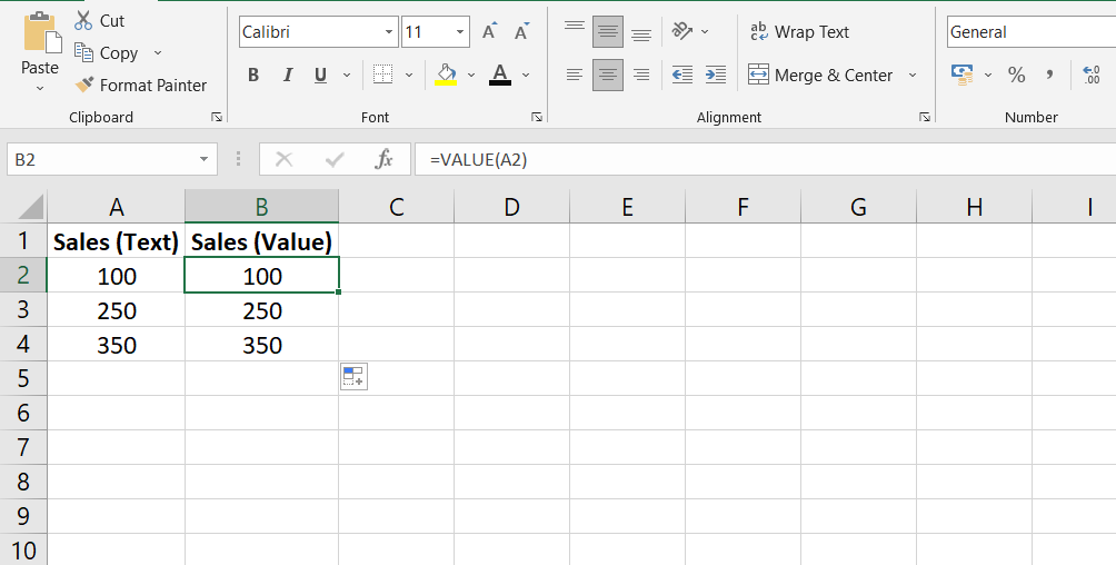
The syntax for the VALUE function is as follows: =VALUE(text).
For example, you have a dataset where sales values are stored as text in column B. You would use the VALUE function to convert these text values to numbers for further analysis. The formula =VALUE(B2) would be applied in a separate column to convert the text in cell B2 to its corresponding numerical value.
UNIQUE function
The UNIQUE function is a powerful feature available exclusively in the Microsoft 365 version of Excel. It enables users to extract a list of unique values from a given range, making it easier to analyze and work with distinct data.
To use the UNIQUE function, you must provide three parameters: the array or range from which you want to extract unique values, whether you want to check uniqueness by column or row, and whether you want only unique values or distinct values (occurs only once).
The syntax for the UNIQUE function is as follows: =UNIQUE(array, by col, exactly once).
For example, let's consider a scenario where you have a list of product sales and you want to extract a unique list of product names. Excel will automatically generate a spilled range with only the unique product names by applying the UNIQUE function and providing the range containing the product names, such as =UNIQUE(B2:B15).
This spilled range dynamically adjusts as new unique values are added or existing values are modified. You can then use these unique values for further data analysis or calculations. For instance, you can utilize functions like SUMIFS to calculate the total sales for each unique product name.
FAQs
What are the 10 Excel functions?
The 10 Excel functions are SUM, AVERAGE, COUNT, MAX, MIN, IF, VLOOKUP, CONCATENATE, DATE, and PMT.
What are the 5 basic Excel skills?
The 5 basic Excel skills include navigating through spreadsheets, entering and editing data, formatting cells, creating basic formulas, and using functions.
What are some useful functions in Excel?
Some useful functions in Excel include SUM, IF, VLOOKUP, COUNTIF, CONCATENATE, TEXT, TODAY, and PMT.
What are the 5 powerful Excel functions that make work easier?
The 5 powerful Excel functions that make work easier are VLOOKUP, INDEX MATCH, SUMIFS, CONCATENATE, and PIVOT TABLE.
What is the most popular Excel function?
The most popular Excel function is probably SUM, which adds up values in a range of cells.
Final Thoughts
Excel is a powerful tool for data analysis, and understanding the most important functions is key to maximizing its potential.
The top 10 essential Excel functions covered in this resource provide the fundamental tools for performing common data analysis tasks, making calculations, and manipulating data effectively.
By mastering these functions, users can enhance their Excel skills, improve efficiency, and unlock the full capabilities of this versatile software for data-driven decision-making.
One more thing
If you have a second, please share this article on your socials; someone else may benefit too.
Subscribe to our newsletter and be the first to read our future articles, reviews, and blog post right in your email inbox. We also offer deals, promotions, and updates on our products and share them via email. You won’t miss one.
Related articles
» Guide to Using COUNTIF Function with Examples for Index Match Excel Formula
» Mastering Excel Formatting with the TEXT Function - A Guide
» How to Use the CONCATENATE Function in Excel: Guide with Examples