
This step-by-step guide will give you the necessary instructions to transform your worksheet and make it visually appealing. Let's dive in and discover how to shade rows and columns in Excel to improve your data presentation.
Table of Contents
- Shading the Cells Using Conditional Formatting
- Shading the Cells Using MOD Formula
- Understanding the MOD Formula
- FAQs
- Final Thoughts
Shading the Cells Using Conditional Formatting
To shade cells using conditional formatting in Excel, follow these steps:
- Open your Excel sheet and select the range of cells where you want the formatting to be applied.
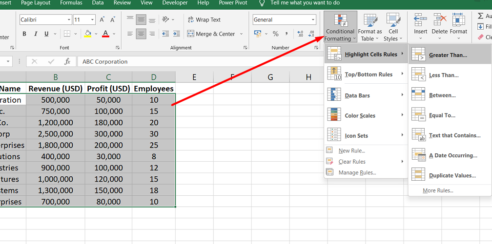
- Go to the Ribbon at the top of the Excel window and locate the "Conditional Formatting" option.
- Click "Conditional Formatting" to open a drop-down menu with various formatting options.
- Choose "Highlight Cell Rules" or "Top/Bottom Rules" to determine how the cells will be highlighted based on their values.
-
When you select one of these options, a dialog box will appear where you can enter the criteria for highlighting the cells.
- For "Highlight Cell Rules," you can specify values that should be highlighted, such as cells greater than a certain value or cells between a range of values.
- For "Top/Bottom Rules," you can highlight the top or bottom percentage or a number of cells based on their values.
- Once you've set the desired criteria, select the preferred formatting style from the available options.
- Click "OK" to apply the conditional formatting to the selected cells.
Using conditional formatting, you can easily shade cells in Excel based on specific values or conditions. This feature lets you visually emphasize important data and make it easier to analyze and interpret.
Shading the Cells Using MOD Formula
To shade cells using the MOD formula in Excel, follow these steps:
- Select the rows or columns that you want to be alternately shaded.
- Click on the "Conditional Formatting" tab in the Excel ribbon.
-
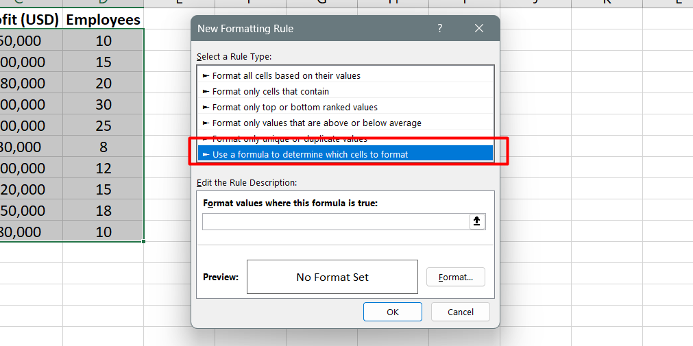
Choose "New Rule," typically the third option from below, to open an extended window for rule configuration.

-
In the rule configuration window, select the option that says "Use a Formula to Determine Which Cells to Format."
-
Enter the MOD formula in the provided space: =MOD(ROW(),2)=0
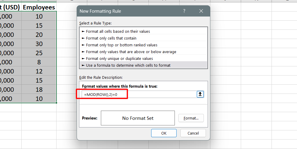
- Format the cells by clicking on the format icon below the formula input space, typically represented as a paint bucket or similar symbol. Choose the desired color and style for the shading.
- Click OK to apply the formatting rule.
After following these steps, the selected cells will display alternately shaded rows based on the MOD formula. The MOD and ROW functions check if the row number is even or odd. If the row number is divisible by 2 (i.e., the MOD result is 0), the formatting will be applied, resulting in alternating shading.
Understanding the MOD Formula
The MOD formula is versatile and can be adjusted to fit different shading requirements in Excel. By replacing 'ROW' with 'COLUMN' in the formula, you can apply the shading to columns instead of rows. Additionally, you can modify the numbers in the formula to achieve different shading patterns.
To shade specific columns instead of rows, replace 'ROW' with 'COLUMN' in the MOD formula.
To change the shading frequency, modify the number 2 in the formula. For example, replacing 2 with 4 will shade every fourth row or column.
Adjust the number in the formula accordingly to start shading from a different row or column. For instance, changing the number 0 to 1 will start the shading from the first row or column.
These adjustments allow you to customize the shading pattern based on your preferences and formatting needs. Excel provides flexibility in utilizing the MOD formula to achieve various shading arrangements, enhancing the visual representation of your data.
FAQs
How do I shade a column in Excel?
To shade a column in Excel, select the entire column by clicking on the column header, then go to the "Home" tab, click on "Fill Color," and choose the desired shading color.
How do I highlight all rows and columns in Excel?
To highlight all rows and columns in Excel, click on the square at the top-left corner of the worksheet where the row and column headers intersect, which selects the entire sheet, and then apply the desired formatting, such as choosing a fill color.
How do I GREY out rows and columns in Excel?
To grey out rows and columns in Excel, select the desired rows or columns by clicking on their headers, go to the "Home" tab, click on "Font Color," and choose a shade of grey.
How do I GREY out rows in Excel?
To grey out rows in Excel, select the desired rows by clicking on their row numbers, go to the "Home" tab, click on "Font Color," and choose a shade of grey.
How do I get GREY lines in Excel?
To get grey lines in Excel, select the cells, rows, or columns where you want the lines to appear, go to the "Home" tab, click on "Borders," and choose a grey border style.
Final Thoughts
Shading rows and columns in Microsoft Excel is a simple yet effective way to enhance data visualization and make your worksheets more visually appealing. By using conditional formatting, you can apply formatting styles based on specific criteria or values, highlighting the cells that meet those conditions.
This allows you to draw attention to important data and make it easier to analyze. Alternatively, you can utilize the MOD formula to create alternating shading patterns for rows or columns.
This provides flexibility in customizing the shading based on your preferences. Whether you choose conditional formatting or the MOD formula, shading rows and columns in Excel can significantly improve the readability and presentation of your data.
One more thing
If you have a second, please share this article on your socials; someone else may benefit too.
Subscribe to our newsletter and be the first to read our future articles, reviews, and blog post right in your email inbox. We also offer deals, promotions, and updates on our products and share them via email. You won’t miss one.
Related articles
» How to Delete Multiple Rows in Excel: A Quick and Easy Guide
» Transpose Excel columns to Rows in Excel chart
» How to Limit Rows and Columns in an Excel Worksheet