Excel is the most powerful tool for analyzing large sets of data. However, to keep your headers on screen, you need to learn how to freeze a row in Excel on Mac. That way, you won't lose sight of valuable data on your top row or column when scrolling your spreadsheet.
Assuming you have numerous rows of data in Excel. When scrolling down, the headers disappear. Thus, it is difficult to ascertain the values contained in your columns. The solution is to freeze rows and ensure that headers stay inview as you scroll the spreadsheet.
This guide teaches you the simple steps of how to freeze a row in Excel for Mac.
Freezing the First Row in Excel 2011 for Mac
Method 1: Freeze Panes
More columns and rows translate to a complex problem of losing sight of data. In such a scenario, you must understand how to freeze a row in Excel 2011 for macOS. Use these easy steps to make sure your rows stay in place regardless of where you scroll. However, take note that these steps also apply when freezing columns as well.
- First, open your spreadsheet in Excel.
Tip:Ensure that your spreadsheet is in Normal View. Click on View. Then select Normal to get a normal View.
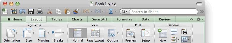
- Next, select the Layout Menu located on the toolbar.
- Now, click on theFreeze Panesbutton.
Excel gives you four options to choose from. However, in Mac, the Freeze Panes options are not explained, unlike in Windows. Here are your options:
- Freeze Panes:Use this option to lock your selected rows or columns other than the top row and left column.
- Freeze Top Row:With this option, you can only see the top row as you scroll the remainder of the spreadsheet.
- Freeze First Column:Clicking this option makes the first column visible as you scroll the remaining spreadsheet.
- Unfreeze:This option unlocks all the columns and rows. However, unfreeze is detached from other options in Mac.
- Click Freeze Top row from the pop-up Window to lock your row.
Tip:This option is located in the right-hand corner of your spreadsheet.
Once you choose this action, the top row stays in place as you scroll down the rest of the spreadsheet. And when you scroll back up, the top row is still intact. Impressive, right?
Freezing the Rows of your Choice
Do you want to freezeas many rows as possible? It's possible. However, you must start with the top row when freezing. If you're going to freeze rows of your choice, follow these simple steps:
- First, click the cell below the row that you want to lock.
- For instance, if you desire to lock the first three rows, then click cell A4. Now select Layout and choose the Window group.
- Click on the Freeze Panes button and select Freeze Panes from the drop-down menu.
Everything above Cell A4 or any other active cell is frozen. A grey line is displayed along the cell gridlines when you apply the Freeze option. After that, the rows of your choice remain on screen as you scroll the rest of your spreadsheet. Take note that these steps are similar when you want to learnhow to freeze a row in Excel for Mac 2019.
How to Freeze Columns in Excel for Mac
But what if you want to freeze columns instead? If you desire to see specific columns of your spreadsheets all the time, it's straightforward.
- First, open your Excel spreadsheet.
- Select the columns you want to freeze.
- Now, click the Layout tab on the toolbar.
- Navigate to the Window group and click the Freeze Panes button.
- From the drop-down menu, select Freeze Panes.
The selected column will be locked or frozen as portrayed by the grey lines. That way, you can see your column as you scroll across the spreadsheet.
How to Freeze the First Column and the Top Row
Probably you want to lock the first column and the top row of your spreadsheet simultaneously. Make sure that you select the cell below the top row and to the right of the first column.
- First, select Cell B2.
- Next, click the Layout tab and navigate to the Window group.
- Click Freeze Panes ribbon.
- Now, from the drop-down menu select Freeze Panes
Applying this action freezes the top row of your spreadsheet and the first column regardless of where you scroll.
Method 2: Split Panes
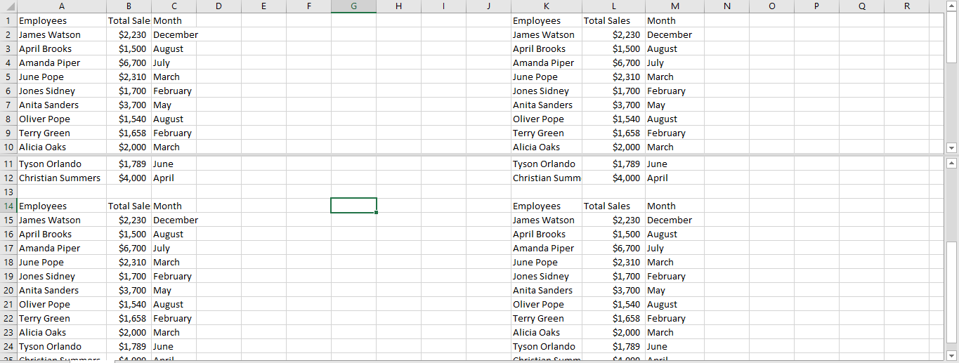
Alternatively, you can use the Split option to freeze and separate your rows into different worksheets. By freezing Panes, you can keep particular rows or columns visible as you scroll your spreadsheet. However, just as the name suggests, splitting panes divides your worksheet area into two or four scrollable regions. What's more, scrolling one section keeps the cells in place or locks them.
Instead of wasting time scrolling the spreadsheet back and forth, just split the spreadsheet into two scrollable panes. Splitting rows makes it possible to view the top and lower panes as you scroll your worksheet. Here's how
- First, open your desired spreadsheet
- Next, select the row below and to the right of where you want to split.Select row 11 cell A11 to split row 10
- Next, click the Layout tab of the ribbon.
- Select the Window group and choose the Split button
Excel gives you two areas that are scrollable and which contain the whole worksheet. That way, you can work with extensive data that does not appear on the screen at the same time.
To unlock or unfreeze your row, click the split button again.
How to Unfreeze a Row in Excel
Having learned how to freeze a row in Excel for Mac, it's also possible to unfreeze a row.
Here's how:
- Click the Layout Menu
- Next, select the Unfreeze Panes
Once you click on the Unfreeze Panes, then all the rows will be unlocked. However, once you choose the Unfreeze Panes option, it's only then that it becomes visible on your spreadsheet.
If working with broad data is frustrating, why don't you choose to freeze or split your rows? Knowing how to freeze a row in Excel for Mac or split rows makes your headers visible on your screen all the time. What's more, it saves you hours of work as you scroll down the rest of the spreadsheet as you compare data.
If you're looking for a software company you can trust for its integrity and honest business practices, look no further than SoftwareKeep. We are a Microsoft Certified Partner and a BBB Accredited Business that cares about bringing our customers a reliable, satisfying experience on the software products they need. We will be with you before, during, and after all the sales.